The total subsea search for MH370 comprised more than 240,000 km2 of seabed in the Southern Indian Ocean (SIO) along the 7th arc, which is derived from the metadata from the last transmission from MH370’s SATCOM terminal. The search of the first 120,000 km2 was managed by the Australian Transport and Safety Bureau (ATSB), and included the areas that Australia’s Defense Science and Technology Group (DSTG) deemed most likely as the Point of Impact (POI). The ATSB’s subsea search along the 7th arc extended in latitude from 39.4 S to 32.8 S, varying in width from 130 km at the southern end of the search area to 40 km at the northern end.
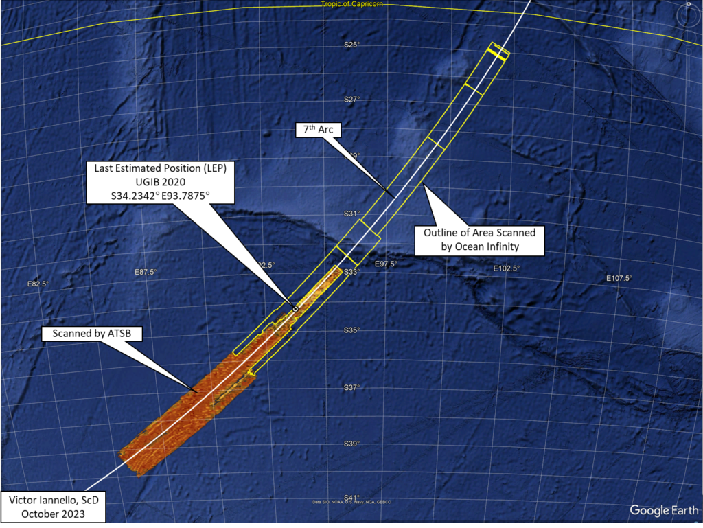
An additional 120,000 square kilometers of seabed was scanned by Ocean Infinity (OI) using a fleet of autonomous underwater vehicles (AUVs). OI extended the length and width of the ATSB’s search so that a full 110 km width was scanned along the 7th arc north to a latitude 31.5 S. The search area was then narrowed to a width of 84 km and extended north along the 7th arc to a latitude of 24.8 S.
Despite this unprecedented large search in the area deemed most likely to find the debris field, the search was unsuccessful. So why wasn’t MH370’s debris field identified? There are only three realistic possibilities:
- The aircraft was manually piloted after fuel exhaustion and glided beyond the area that was previous searched. Although the final BFO values suggest an increasingly high rate of descent that would certainly have resulted in an impact within kilometers of the 7th arc if there had been no further pilot inputs, there is a possibility that the pilot arrested the steep descent and transitioned into a long, efficient glide.
- The point of impact (POI) occurred along the 7th arc further south than 39.4 S or further north than 24.8 S. For instance, although the statistical match to the satellite and drift model data is not as strong, Ed Anderson has discovered an acoustical event along the 7th arc at 8.4 S that he believes is related to MH370. Meanwhile, Paul Smithson believes an impact further south than 39.4 S is within the uncertainty limits of the fuel consumption and drift models, and should not be excluded.
- The debris field lies on the seabed within the area already searched, but was not identified due to challenging terrain, low quality data, or equipment issues.
Here we address the third possibility. In particular, we again consider whether the debris field might be located in the high probability search area previously identified, which is in proximity of the last estimated position (LEP) calculated in the UGIB 2020 study. We further consider whether parts of MH370 were detected but were never fully investigated because they were not part of a larger debris field.
In the figure below, the two inner yellow lines show the approximate limits of the area searched by the vessel GO Phoenix (under contract with the ATSB), and the outer lines show the limits of the Ocean Infinity search area. Also shown in the figure are olive-green areas which represent areas that were not scanned by GO Phoenix’s towfish due to steep terrain. The outlines of these and other areas of missing or low-quality data were made available by Geoscience Australia.
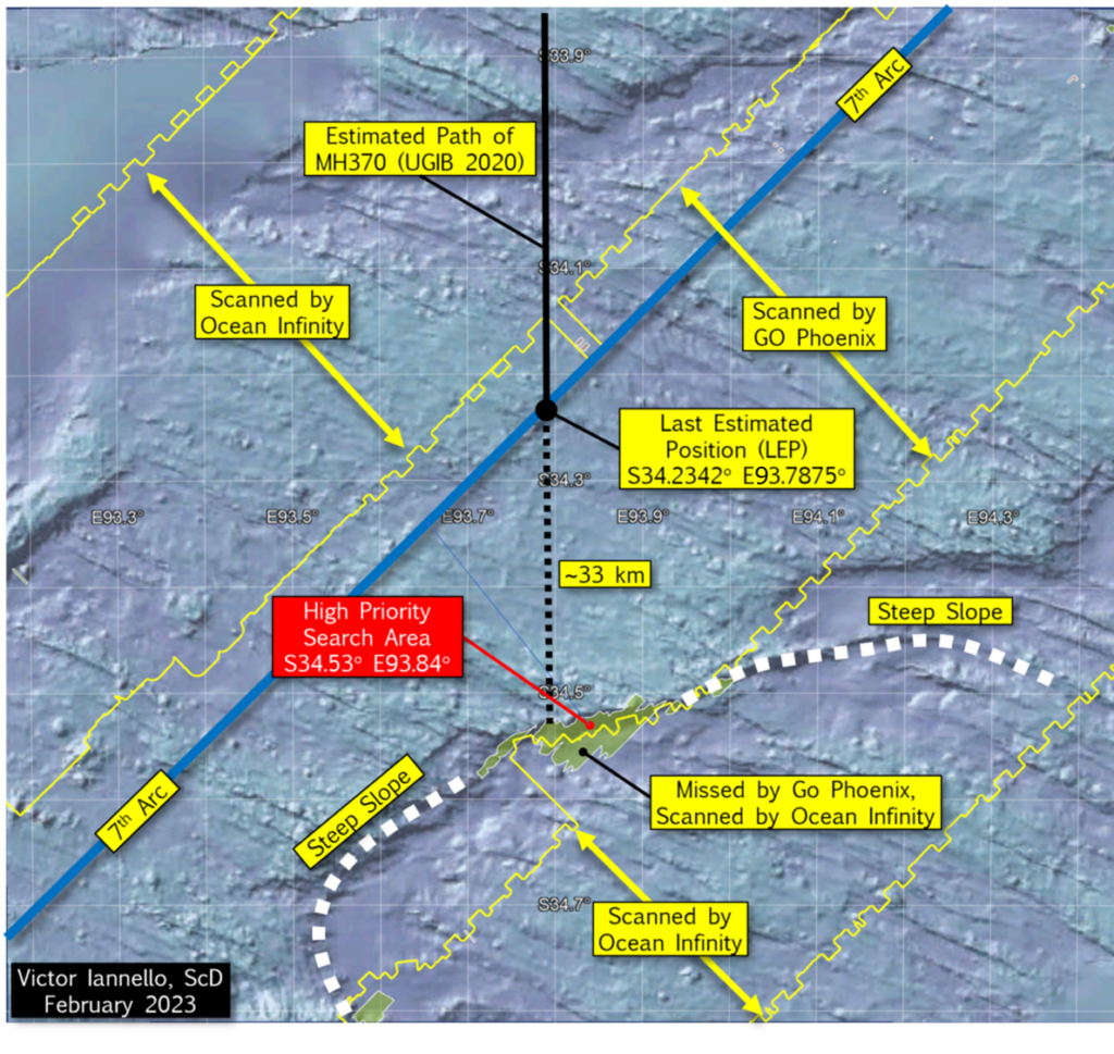
There is a steep slope to the south of the LEP, and the portion of the steep slope that was not scanned by the GO Phoenix towfish is about 60.3 km2. Of this, about half was later scanned by Ocean Infinity AUVs, leaving about 30.5 km2 of seabed surrounding S34.53° E93.84° that was never scanned. We designated this area as a “High Priority Search Area”, and it may be here that the debris field lies.
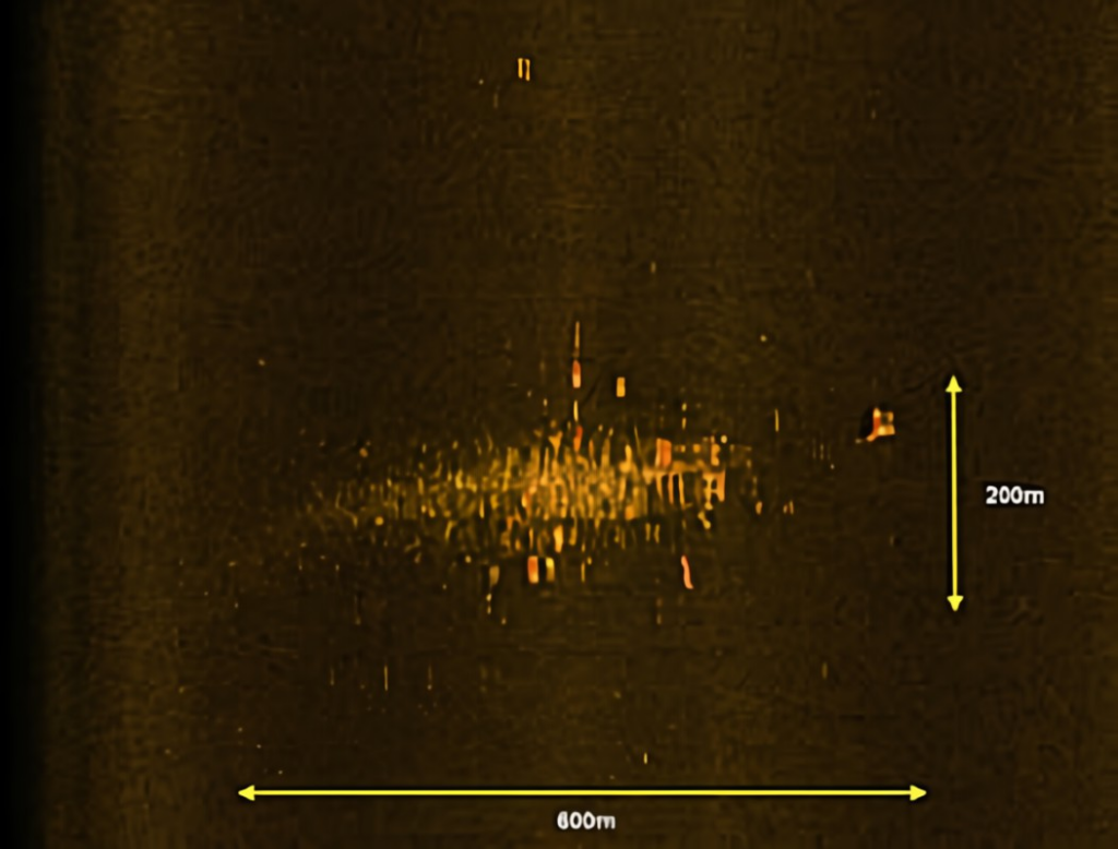
The subsea search for aircraft wreckage that many deem most similar to the search for MH370 was the search for Air France 447 (AF447), which was an Airbus A330 that crashed off the coast of Brazil in June 2009 in around 3000 m (9,800 ft) of water. Floating remnants of the aircraft were found within 2 days of the crash, but the subsea search was not successful in locating the debris field until April 2011, about 2 years after the crash. The sonar image from the debris field, which measured around 200 m x 600 m, is shown below.
AF447 is believed to have impacted the ocean surface without breaking up in flight and with a nose-up attitude. As such, the debris field that AF447 generated may be significantly different from the debris field created by the impact of MH370, as the final two BFO values suggest a high downward acceleration of 0.7g, and descent rates greater than 15,000 fpm. Without pilot intervention, MH370 possibly entered the water at a descent angle greater than 45 deg and at an airspeed approaching or exceeding Mach 1.
The debris from MH370 may more closely resemble the debris from SilkAir 185 rather than the debris from AF447. SilkAir 185 was a Boeing 737 that crashed into the Musi River near Palembang, Sumatra, Indonesia in December 1997. The aircraft experienced a rapid, nearly vertical dive that the US NTSB attributed to control inputs from the captain. During the high speed descent, parts of the control surfaces, including a large portion of the tail section, separated from the fuselage due to the high aerodynamic forces from the high speeds. The airspeed of the fuselage before impact is believed to have exceeded Mach 1.
SilkAir 185’s debris was found in two areas: the main debris field of around 60 m x 80 m at the bottom of the Musi River, which was only 8 m (26 ft) deep; and other larger debris, mainly flight control parts that separated before impact, that were widely scattered on land no closer than 700 m (2,300 ft) from the main debris field. According to the accident report, due to the high energy of the impact, the parts recovered from the river were “highly fragmented and mangled on impact” which made identification difficult.
If MH370 experienced the rapid descent suggested by the final BFO values, then it is probable that the fuselage broke apart before impact, and also probable that many large parts would be found outside of the main debris field. The flaperon recovered on Reunion Island is a good example of a flight control part that may have separated before impact. We would also expect the main debris field to be smaller in extent than for AF447, and within that debris field, the debris to be smaller and more difficult to identify. For instance, for the case of SilkAir 185, the landing gear was identified only by its subcomponents (struts, landing gear door actuators, wheels, brakes, tire pieces, etc.). This counters conventional wisdom that says that aircraft engines and landing gear should be among the easiest parts to identify by sonar on the seafloor, as it was the case for AF447.
The subsea search for MH370 was focused on finding the main debris field at the expense of identifying other parts that may have separated. For the search phase conducted by GO Phoenix, reports were written for a total of 45 “contacts” (observable features in images) that merited a further review. All the contact reports are compiled here. Of these 45 contacts, 24 contacts were within 100 km of the LEP, 10 contacts were within 50 km of the LEP, and 4 contacts were less than 25 km from the LEP. The locations of the contacts are shown in the figure below.
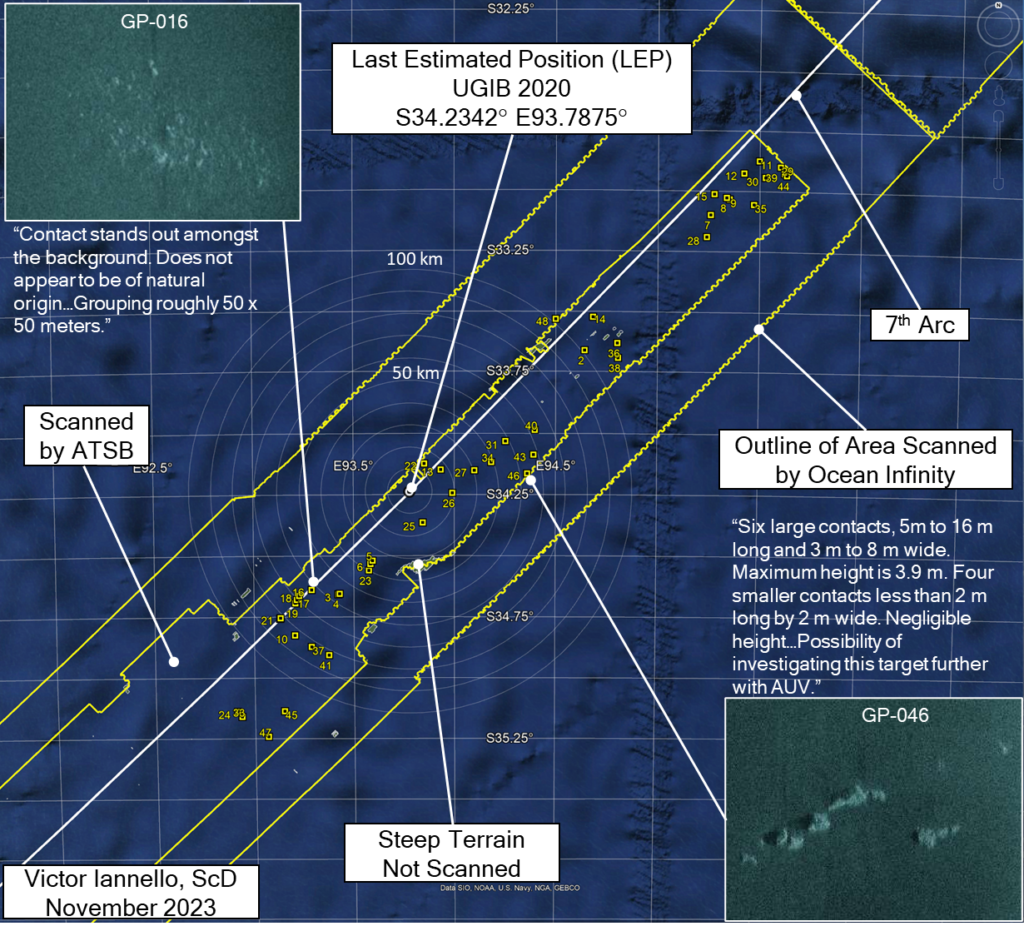
Of the 45 contacts, 11 (GP-002, 016, 018, 019, 021, 025, 026, 028, 030, 031, 047) were described in the reports with phrases like possibly “man-made”, “not geological”, or “not of natural origin”, and one (GP-046) was considered for further investigation with an AUV, which seems to have never been done. Of course, many of the man-made objects on the seafloor could be marine debris from sea vessels unrelated to MH370.
Andy Sherrill is an experienced ocean engineer who has conducted deep water search and salvage operations for a number of missions. He was a key member of the team that reviewed the sonar data for the subsea searches for MH370 that were conducted by the ATSB and Ocean Infinity. Andy was also part of team that identified the debris field for AF447 off the coast of Brazil as well as part of the team that found Argentina’s ARA San Juan submarine. Andy graciously offered these comments as to why many of the MH370 promising contacts were never investigated further:
“Typically, if there were small isolated objects that appeared to be man-made and marked as a target, but nothing else was of interest within several kilometers then we did not investigate further.
We certainly took into account if the debris field did not look like AF447 or any others, however there still needed to be enough debris to be at least a fair amount of the aircraft to warrant further investigation.
Sure a small part of the plane could have drifted and sunk, but we were looking for the main field. A decision was made to focus on finding the main field of debris, not just one small piece – and likely all of those “potentially man made” contacts are from passing vessels given there was no associated debris within several kms.
Having said that, there is always a chance it [a tagged contact] could be from MH370, but based on our assessment the time it took to investigate each of these small contacts was not worth taking vs searching new areas.”
Discussion
As the final BFO values, the lack of IFE log-on, and the end-of-flight simulations all suggest a high speed impact close to the 7th arc, a high priority should be to completely scan the areas closest to the 7th arc. MH370’s debris field may be smaller in area, consist of smaller parts, and be much more difficult to identify than searchers were anticipating. It’s also possible that the debris field is located in an area that was not fully searched due to challenging terrain, low quality data, or equipment issues, such as the steep slope identified above as the high priority search area due south of the LEP. As such, the investigation of many of the contacts previously identified becomes more important, as one or more of these contacts could be parts of MH370 that separated before impact. It’s also possible that one or more contacts are part of a less conspicuous debris field.
We again acknowledge that with pilot inputs, it is possible that MH370 glided after fuel exhaustion beyond the areas that were previously scanned. Therefore, searching wider along the 7th arc should also be part of the search plan if pursuing areas close to the 7th arc is unsuccessful in locating any of MH370’s wreckage.
Update on Nov 3, 2023
Andy Sherrill offered these additional comments:
“We did get rerun over GP16, and collected some higher frequency AUV SSS on that one. Looks highly likely to be geologic in my opinion.
We did not reacquire any more data over GP46, however that one looks very similar to GP16 and I would still classify it as highly likely to be geologic.”
Tags: AF447, debris field, MH370, SilkAir 185, sonar, subsea
@VictorI. Your bottom diagram indicates that there were 46 “man-made”, “not geological”, or “not of natural origin” objects detected by GO Phoenix, yet none in the adjacent OI area. In particular the sharp presence/absence at the go Phoenix north eastern boundary is striking.
This absence of ‘overlap’ between the two areas suggests either that OI has not disclosed such detections or those it detected were confirmed to be of no interest.
If the latter, that would weaken the chances that the GO Phoenix detections could prove of interest. If on the other hand any were left uninvestigated by OI on the same grounds as GO Phoenix, it would be of interest if they would disclose where these were.
Also, if in fact none such were detected by OI near the GO Phoenix area perhaps the two had different sensor sensitivities or detection criteria?
I am convinced that someone was at the control at the end of the flight as all data show that the aircraft was piloted during the 1st hour of the disappearance. Why should not be it the case at the end?
The image with all detected debris is interesting.
But I find your end point too close from the 7th arc. In my opinion, a huge wreckage as a Boeing 777 has highly reflective parts especially engine and gear parts. And more likely with a field debris. So the detection of it should have been highly probable with a not so high resolution.
For me, we have to search further south as the aircraft was glided not so far from the already searched area. That’s what I have suggested for years and this is what suggests the latest study of Patrick Blelly and Jean-Luc Marchand. And I agree with their analysis.
@David: 1) Only 11 of the 45 contacts were described as man-made. Many were described as geological, and for many, the description did not specify whether the investigators believed the objects were man-made or natural. 2) We don’t have contact reports from OI, which is why there are no contact locations in the areas searched by OI.
@Gilles Diharce: We don’t know if there was a controlled glide after fuel exhaustion, despite the strong beliefs that some have claiming with certainty that it did or did not occur. The BFO values at the final log-on suggest a progressively steep descent, and the shattered parts from the cabin interior suggest a high speed impact. If there was a glide, it would mean a dive, a glide, and a final dive. It’s not impossible that this occurred, but it is far from certain that it did. (You might believe the flaperon was damaged during a controlled ditching, but even in that scenario, there was a dive before the controlled glide.)
You believe that it is unlikely that MH370 was missed during the subsea search, despite the data holidays and man-made contacts that were identified but not investigated further. I suggest you read a previous blog post describing OI’s search for ARA San Juan, where the submarine was missed during the first pass.
Again, I am completely in favor of searching wider than what was previously searched to cover the possibility of a long glide after fuel exhaustion. However, I would advocate doing this after completing the search closer to the 7th arc, as there is much less area to cover, and there are some interesting areas and contacts to further investigate.
Andy Sherrill offered these additional comments:
“We did get rerun over GP16, and collected some higher frequency AUV SSS on that one. Looks highly likely to be geologic in my opinion.
We did not reacquire any more data over GP46, however that one looks very similar to GP16 and I would still classify it as highly likely to be geologic.”
From the Inspector General of the US Dept of Transportation:
California Pilot Indicted for Interfering With a Flight Crew
On October 18, 2023, a grand jury in the U.S. District Court for the District of Utah indicted Jonathan J. Dunn for interfering with the crew of a commercial airline flight.
The indictment alleges that, on or about August 22, 2022, Dunn, the crew’s First Officer, interfered with the performance of a crew member by using a dangerous weapon to assault and intimidate the Captain. Dunn was authorized to carry a firearm through the Transportation Security Administration’s Federal Flight Deck Officer program. After a disagreement about a potential flight diversion due to a passenger medical event, Dunn told the Captain they would be shot multiple times if the Captain diverted the flight.
DOT-OIG is conducting this investigation with the Federal Bureau of Investigation with substantial assistance from FAA.
https://www.oig.dot.gov/library-item/39680
@Victor
@Gilles
I am out-voted 99-to-1 but I do not feel an active pilot flew straight to 34-38s with little or no maneuvers just to run out of fuel at Arc7 at high altitude and manage that situation. I do believe Active Pilot: the BFO at Arc7 is very indicative of active pilot making a descent. We are not expecting a ghost flight to dive, and especially not to fly level for 2-minute period and then dive. We seem to be systematically ruling out slow down after Arc5 due to straight flight advocacy. Also everyone is ruling out fuel remaining at Arc7, and that may be wrong assumption too.
What’s coming in a podcast soon probably is Jeff Wise is going to say conspiracy theorists are correct because $300Million of searches failed to find MH370 as a ghost flight ending near Arc7. I am going to say — MH370 is still in the SIO — but the basic assumptions (straight flight to fuel exhaust at Arc7) are probably wrong.
There’s maybe a mistake in this sentence: ”Of these 45 contacts, 24 contacts were within 100 km of the LEP, 10 contacts were within 25 km of the LEP, and 4 contacts were less than 25 km from the LEP.”
Does the linked report include all of Go Phoenix’s contacts? If it does, I find it surprising that the total number is this low and includes only one(?) level 2 contact while the rest are level 3. Maybe the standards of classification were different between Phoenix and Fugro.
Relevant section from the 2017 ATSB report:
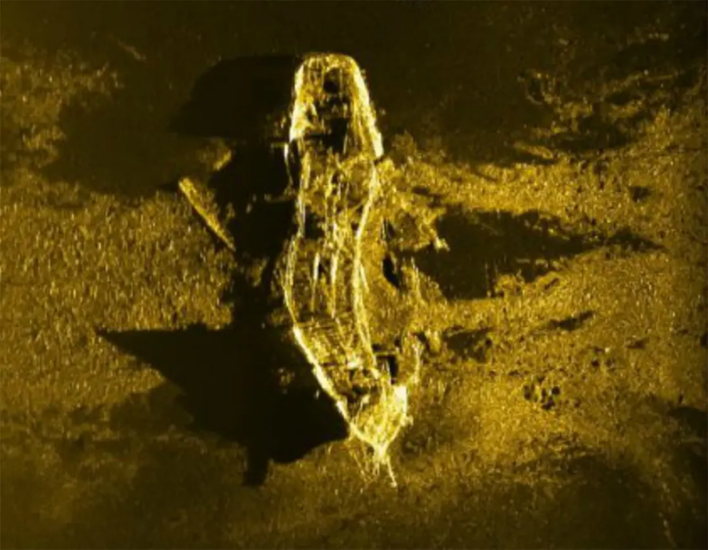
”Sonar contacts (anomalous features) identified in the sonar data were classified in three ways: level 3 contacts were marked but assessed as unlikely to be related to the aircraft, level 2 contacts were marked but assessed as only possibly being related to the aircraft, and level 1 contacts were of high interest and warranted immediate further investigation. There were 618 level 3 contacts, 41 level 2 contacts, and two level 1 contacts identified and reported. The two level 1 contacts were investigated and found to be iron and coal remains of a wooden shipwreck and the other was a scattered rock field. In total, four shipwrecks were found. Throughout the search 82 separate sonar contacts were investigated and eliminated (as being related to MH370) by the AUV, ROV, or deep tow vehicles.”
This link has all the contact reports for the ATSB subsea search:
https://dapds00.nci.org.au/thredds/catalog/iy57/documents/contact_reports/catalog.html
The link I provided in the article is a compilation of only the GO Phoenix contacts. There are many more Fugro contacts.
@Victor
I am more cautious about the last BFO. It seems showing a steep dive but this doesn’t mean that nobody was piloting the airplane at the end. It is not so far certain that this occurred too. It depends on what hypothesis you consider and I agree that we can have a different opinion on this aspect.
Of course, some interesting points may need to be investigated further. But I think it is unlikely as I am confident on professionals who worked on it to consider if it is relevant or not.
Despite our different analysis of this last moment of the MH370, we all have the same goal: find the plane to expect solving this mystery and terminate all conspiracy theories on it.
This is not a course for a winner.
We want the truth for the families.
@Gilles said: I am more cautious about the last BFO. It seems showing a steep dive but this doesn’t mean that nobody was piloting the airplane at the end.
I never said that the final BFO values prove the aircraft was unpiloted. There are two ways to achieve the downward acceleration of 0.7 g:
1) A nose-down input from a pilot
2) A banked, steep descent with no pilot inputs
However, if there were pilot inputs and the aircraft is beyond the area that was already searched, it would mean there was a dive-glide-dive sequence. It’s possible, but that’s the sequence that would have occurred.
We want the truth for the families.
Of course we do. There is not a person that contributes to this blog that is not in pursuit of the truth.
I will once again say that I fully acknowledge that it is possible there was a long glide. I am only saying that the next search should finish the job of searching near the arc before extending wider. Is that really controversial? Why is there pushback?
@victor @Don @Gilles
Thanks for the new post.
We think you are right to raise Point 1 including a glide and a recovery of the fast rate of descent. It is an essential one. We investigated and described this as Descent Scenario #2 in Appendix 1 of our March report (https://www.mh370-caption.net/wp-content/uploads/3-known-trajectory-and-recalculated -trajectory.pdf) and also explained it to Don (and others 🙂 at the RAeS conference in London a few weeks ago (https://www.youtube.com/watch?v=CjjySxoo_AQ ).
The other Descent scenario 1 also includes a glide.
From these one can deduce the shortest potential distance from Arc7 to the POI which is between ~42 Nm and ~67 Nm (from FL300). We therefore think that the strip of sea to look further than Arc 7 is wider than the few kilometers that you propose. It would be even wider if started at a higher flight level.
Videos of the respective simulation sessions for each scenario are available here: https://youtu.be/4gdZAFg7wJI and https://youtu.be/x7ezFNFca-A
Sherrill’s comment:
”but based on our assessment the time it took to investigate each of these small contacts was not worth taking vs searching new areas.”
In general, this argument is still just as valid as it was then. And it could even be argued that, as search technology has improved (lower cost per km²), the cost of checking a contact (in terms of wasted km²) may have gone up. However, if certain latitudes can be prioritized based on probability, it may make more sense to check the contacts in those areas.
So when you say ”a high priority should be to completely scan the areas closest to the 7th arc”, do you mean the whole previously searched 7th arc or some more prioritized latitudes (e.g. S33-36)? And by ”completely scan”, do you mean checking contacts and previously missed areas, not researching already searched areas?
@Victor
The more important thing is to obtain the continuation of the search.
If the official accepts searching on both areas (yours and Blelly/Marchand’s), I think we have a good chance to solve this affair.
But we have to be aware that some points of this disappearance will still remain unexplained. We will never know what really happened in the cockpit at the time of the disappearance as it would have been erased in the CVR unfortunately.
🤞🤞🤞🤞
@Jean-Luc Marchand: We therefore think that the strip of sea to look further than Arc 7 is wider than the few kilometers that you propose.
Where did I say the search should be constrained to a few kilometers from the 7th arc? With a long glide from a high altitude, the glide could have been 140 NM! The search area we proposed in the last post included the possibility of a long glide (Zone 3).
I will yet once again say that I fully acknowledge that it is possible there was a long glide. I am only saying that the next search should finish the job of searching near the arc before extending wider. Is that really controversial? Why is there pushback?
@eukaryote234: I wouldn’t suggest researching everything already searched. As I said in the discussion section of the post:
It’s also possible that the debris field is located in an area that was not fully searched due to challenging terrain, low quality data, or equipment issues, such as the steep slope identified above as the high priority search area due south of the LEP. As such, the investigation of many of the contacts previously identified becomes more important, as one or more of these contacts could be parts of MH370 that separated before impact. It’s also possible that one or more contacts are part of a less conspicuous debris field.
So basically, search data holidays (including challenging terrain not searched) and promising contacts. I would prioritize the GO Phoenix portion of the search because that’s where the statistical match to the data is best (i.e., UGIB 2020).
Then search wide, which is a much larger area and will take a lot more time.
@Gilles: Doesn’t the area we recommended to search in the last post include the area that Marchand/Blelly are now recommending to search?
One thing that Ocean Infinity learned from the ARA San Juan search was that you ignore canyons at your peril. It seems empirically obvious – as undersea currents drag things, they’ll get caught somewhere, most likely within a geological feature. The GO Phoenix and Fugro searches of the original area scanned the high-priority area in the same way that Ocean Infinity scanned the San Juan high-priority area, not pausing to investigate areas where the debris field might well have got stuck.
We have lots of evidence that suggests the wreckage is quite likely pretty close to the arc and pretty close to the LEP. Surely what makes the most sense is to search the areas in that zone we know we haven’t looked? It’s not just that cliff, there are other smaller areas like the subsea canyons that haven’t been carefully investigated.
@Rob Moss: I agree 100%. I don’t understand the pushback to completing the search close to the 7th arc before expanding it wide.
FWIW I also agree (with Rob Moss and Victor last 2 posts).
Regarding Rob’s comment:
« One thing that Ocean Infinity learned from the ARA San Juan search was that you ignore canyons at your peril. It seems empirically obvious – as undersea currents drag things, they’ll get caught somewhere, most likely within a geological feature. »
I was just about to put this very same questions to the subsea experts here:
Are there typically currents around canyons which would pull sinking objects (such as MH370 debris) into canyons so that there is a HIGHER probability of the debris ending up in a canyon (than around it)? Or are these canyons rather stationary zones without much water movement from/into them?
In the former case, Rob would be right that the chance of finding the debris in data holidays due to difficult terrain would be higher than usual.
@VictorI:
Thanks for including my 370Location.org candidate site into your recent paper. I continue to research the MH370 acoustics every day, and have had some recent progress in detecting weaker events using spectral whitening and phase alignment methods applied to beamforming.
No pushback from me on searching targets near the 7th Arc. I suggest resuming the search wherever a narrow track can be followed, consistent with the 7th Arc. That includes unpiloted tangents that some have bet their houses on, and also untriangulated hydrophone bearings from Cape Leeuwin that could be mapped when returning to Perth from a sortie.
My concern about the current paper is that a focus on isolated small sonar targets is pegged to the theory that these pieces of debris would have separated before impact due to “flutter” from a high speed dive, and thus not part of the expected debris field.
I believe the flutter theory was first proposed within a day of the Flaperon being found, to explain the trailing edge damage (and to be consistent with BFO).
Additional found debris adjacent to the Flaperon indicates that the flaps were retracted, which for some has confirmed an unpiloted high speed dive.
The paper compares to AF447 as a slow impact to emphasize how MH370 debris might be highly fragmented due to a supersonic impact.
Let’s look a bit closer. AF447 was descending from high altitude in a 110% full thrust nose-up stall at 108 knots ground velocity and 108 knots downward velocity for vector impact of 152 knots.
The BFO approximation of vertical speed near the last ping was 15,000 fpm or 148 knots. We don’t know the forward velocity. You mention that glide-dive-glide is a possibility. A steep dive has been ruled out when my analysis showed that the last sat pings were at normal signal strength, showing that the attitude of MH370 was not outside the ability of the SATCOM unit to optimally steer the phased array antenna as in normal operation. (No vertical dive, steep bank, or inverted flight).
Trailing edge damage appears very similar on all the debris items found – flaperon, ailerons, horizontal stabilizer. The supersonic flutter theory requires that all these pieces oscillated so violently that they lost their trailing edges in flight and then further detached in unison from the airframe so that they were *not* damaged on impact.
I have not been able to find any examples of violent trailing edge flutter in large aircraft. What I’ve found is flapping and violent twisting of the wings along the chord (wingspan), which didn’t cause all the trailing edge airfoil parts to spontaneously eject.
So, let’s consider the possibility that MH370 was nose-up at lower speed when it hit the water to account for the flaps-up trailing edge damage. Rupture of the fuselage forward of the wings is not inconsistent with the interior debris that has been found.
@Peter Norton:
I don’t expect that there will be significant currents near the seafloor, which includes canyons. Surface currents are driven by winds, and deeper currents by thermal differences. At the abyssal seabed, it is considered quiet – although researchers have documented “storms” where currents approach 0.5 m/sec. Compare that to a max 2 m/s surface current around the 7th Arc.
Now consider the descent rate of debris. It is dependent on the density of an object, including entrained air and water. From the surface, a large fuselage section could sink with captured air pockets. As it sinks, any air would be compressed to an insignificant amount, and the water contained within the structure would add to its mass. I believe this is why the acoustic recordings from a dozen hydrophones and some 45 seismometers were able to pick up the seabed impact of MH370.
If we assume a 4 m/s average velocity for sinking debris, that’s about 15 min to descend to 3400m, the depth at the epicenter of the recordings. It also dwarfs any subsurface currents during the descent.
I expect the seabed debris pattern will be very similar to that of Air France 447. I don’t anticipate isolated fragments will be found far from the crash site.
@370Location
I think you have been rather selective in the data that you use to dismiss a steep dive and flutter.
There is ample evidence of the aircraft speed immediately before, and about the time of the second engine flameout. That might be extrapolated to provide an estimate of forward velocity. Then at that speed the descent angle can be estimated to fit with the 15,000fpm descent.
I was one of the early proponents of the possibility of flutter causing the flaperon damage.
There are different types of flutter, and the type of twisting and oscillating that you refer to is not the same as the aerodynamic flutter that the flaperon may have experienced. Aerodynamic flutter does not require supersonic speeds. It can occur at very moderate speeds in all types of aircraft. The Boeing manual describes the possibility of flaperon flutter occurring during engine testing with the aircraft parked on the ground.
The TE damage on the flaperon shows separation along the line of skin fasteners, i.e. along the weakest part of the TE skin structure. Exactly what one would expect with violent aerodynamic flutter, where the magnitude and frequency of the flutter rises to a peak within a couple of seconds.
@Brian Anderson:
Thanks for the info. It’s inspired some fascinating reading about historic aeroelastic stability.
The case of parked flaperon flutter is interesting. I found that turbofan exhaust velocity on the ground can exceed 325 kt, and is likely very turbulent. It also can cause flutter on new B777 horizontal stabilizers:
https://youtu.be/EKeCZ2nDkDU?si=qWO6TFHWtb61YPkK&t=134
We do have a recent example from the China Eastern MU5735 crash and debris photos. Some granular data is here:
https://www.flightradar24.com/blog/china-eastern-airlines-flight-5735-crashes-en-route-to-guangzhou/
The B737 was cruising 455 kt at 29,100 ft when it went into a sudden vertical dive. I don’t know if it was a powered dive. It initially lost airspeed at the beginning of the dive. It reached a peak airspeed of 590 kt as it was pulling up to level out at 8000 ft. Vertical speed also peaked at -30,976 fpm, but that same value is oddly at three different times (it may be a capped reading so the actual vertical speed could have been greater). Debris photos are sparse, but we can see at least a piece of the rudder and wingtip. Neither appear to have any trailing edge damage.
I’m not entirely dismissing flutter and detachment of most control surfaces, just noting that the re-search recommendation in this paper depends on it.
@370Location: China Air 006 (B777) and SilkAir 185 (B737) both loss parts of the tail control surfaces due to flutter at high aerodynamic speeds. In the case of Silk Air 185, the plane broke apart, with parts that separated during the descent found scattered some distance from the main debris field. For China Air 006, the pilots were able to recover and eventually land the plane.
Link to image showing damage to China Air 006:
https://upload.wikimedia.org/wikipedia/commons/8/83/Damaged_empennage_of_China_Airlines_Flight_006-N4522V.JPG
@370Location:
thank you for your reply concerning underwater currents.
@”We did not reacquire any more data over GP46, however that one looks very similar to GP16 and I would still classify it as highly likely to be geologic.”
To my eyes, GP46 also doesn’t resemble any part of a plane.
@Victor Iannello: “a dive-glide-dive sequence”
Why would a pilot interrupt a dive only to plunge into a dive again ?
Or did you mean a “glide-dive-glide” sequence ?
It would seem more plausible to me that a pilot terrified by the dive and shying away from the suicide would pull out of the dive and continue gliding (and therefore avoiding dying) as long as possible.
On the other hand, a dive-glide-dive sequence could be the result of a pilot aborting the suicide dive, gathering up his courage (gliding) and then carrying out the suicide dive on the second go.
So I guess, both scenarios are imaginable and can’t be excluded.
The 7-hours-long suicide run never made much sense to me until I recently listened again to William Langewiesche‘s interview by Megyn Kelly:
https://youtu.be/v_y0A2cheo4
Although I take issue with a lot of things he says, I think he offers a plausible explanation for hours-long suicide flight:
He couldn’t bring himself to do it, but couldn’t turn back after having killed everyone on board. So he essentially had nowhere to go.
https://youtu.be/v_y0A2cheo4?t=1231
But why then does the flight path match the simulator data weeks earlier ?
That’s left unexplained and doesn’t quite match Langewiesche’s theory.
Your thoughts ?
@VictorI:
Thanks for the followup. One crash due to a suicidal pilot, and the other a crew losing control in whiteout after an engine failure, but eventually recovering.
It’s impressive that the CAL006 B747 could still fly level after the tips of its horizontal stabilizer broke off due to flutter. It appears to have been the flapping/twisting type, as there is no sign of damage along the trailing edge besides the missing sections.
I couldn’t find any photos of intact SilkAir185 trailing edges, but it’s clear that much of the tail broke off. No dispute that aeroelastic flutter is a very real effect.
@Peter Norton:
I try to be objective, but my reply was a bit focused on my own work. Seabed currents could elongate the debris field, but the AF447 debris field orientation did align with the track at impact.
@Peter Norton asked: Why would a pilot interrupt a dive only to plunge into a dive again ? Or did you mean a “glide-dive-glide” sequence ?
That sequence was suggested without regard to pilot intentions. The first dive is based on the final BFO values. The glide is based on a potential impact site beyond what was searched. The final dive is based on the shattered parts of MH370 that were recovered, which suggest a high-energy impact. If that sequence actually occurred, your guess is a good as mine as to why.
@Peter Norton
Peter, you asked, “But why then does the flight path match the simulator data weeks earlier ?”
The short answer is that the flight path does not match the simulator data (unless you have an extraordinarily loose definition for the word “match”).
Suffice to say that the sim data is easily one of the most misrepresented and consequently misunderstood items relating to the disappearance. Leaving aside the blazingly obvious discrepancies such as the simulator flight turning left towards the north-west after take-off and MH370 turning north-east, the only real similarity between the sim flight and MH370 is that both ended up in the Southern Indian Ocean.
In the recovered sim session, the Captain was almost certainly simulating the take-off and departure of his then upcoming flight to Jeddah on MH150. This was a route that he hadn’t flown for some three months. The data shows that after what appears to have been a fairly standard instrument departure, the Captain appears to have simulated some sort of in-flight upset that was then followed by his turning the aircraft around, either heading back to his departure airport, Kuala Lumpur, or possibly to the then nearest suitable airport, Medan, Indonesia. This diversion occurs before the aircraft reaches waypoint VAMPI. That first “phase” of the sim session ends there.
After that, he relocated the simulation aircraft to eastern edge of the Bay of Bengal, roughly equidistant from Port Blair and Car Nicobar. He had flown through that region on the MH17 return flight from Amsterdam to Kuala Lumpur just two weeks prior. From the Bay of Bengal location the aircraft is almost certainly not flown south as many portray it, rather the aircraft was almost certainly flown south-east back towards Indonesia/Malaysia.
During this phase the simulator aircraft was almost certainly jettisoning fuel, such that it reached fuel exhaustion somewhere over the south-western extent of the Andaman Sea, near Banda Aceh, Indonesia. The aircraft began a brief unpowered descent after fuel exhaustion had occurred. The second “phase” of the sim session ended at this point, with the aircraft having reached fuel exhaustion somewhere near north-western Sumatra.
After that, the simulation aircraft, already having experienced fuel exhaustion, was relocated to the Southern Indian Ocean about 940 nm south-west of Perth, Australia. Shortly after that relocation, after another brief period of unpowered descent, the aircraft’s altitude was manually adjusted down from its then current 37,650 feet to 4,000 feet.
It is worth noting that the simulation aircraft was a Boeing 777-200LR, not a -200ER as flown by Malaysia Airlines. The LR has a slightly different wing to, and very much more powerful engines than the -200ER so while the simulator offers reasonable fidelity procedurally, it is offers very limited utility for say, fuel planning or flight performance.
@Peter Norton
My 2 cents, I would advise Langewiesche that the pilot may have had every intent to hide the crash site. The home sim data seems to represent an outline the plan (for MH150). After Arc5 there may have been maneuvers (not straight flight). The reason dive-glide-dive scenario seems awkward is that our assumption that an active pilot agreed with us the he should not touch any controls until he ran out of fuel at FL350+ is questionable.
@TBill
Do you sense increased “push-back” recently ?
My two bob’s worth.
The view (long held in some circles with a fervent religious conviction) that the 7th Arc 8-sec BFO’s are an unarguable slam-dunk indication of a rapid and accelerating unrecoverable descent, leading to imminent and certain unscheduled instantaneous disassembly, is (to my eyes) not supported by the published descent profile of Egyptair 990 in this NTSB graphic.
https://upload.wikimedia.org/wikipedia/commons/3/34/Msr990-ntsb-f1.jpeg
It appears 990’s ROD was comparable to, and indeed greater than, 370’s, and note, it recovered from the dive, and actually climbed, before (according to the radar returns) finally crashing.
I feel that those in some circles, although apparently conceding the remote possibility of an active pilot, still can’t really accept any serious consideration of any active pilot scenario, and are only paying lip service to it, because they have far too much capital invested in the history of the unresponsive pilot scenario.
I am far more inclined to accept the French Captain’s recently presented (at the Royal Aero Society in London) descent profile(s). They are credible, and fit what an active pilot could do, and they allow glides far, far away, from the 7th Arc.
Specifically, they credibly allow for a deliberate intent by an active pilot, to carefully and skillfully deposit his aircraft in either of our two chosen “crevices” (or elsewhere).
I think both crevices should be searched.
@Victor Iannello:
Thank you for the clarification. You are probably right that it might be better to disregard psychological aspects and just focus on the data at hand.
@370Location:
Thanks for the follow-up. According to these 2 sources,
“Submarine canyons are hotspots for litter accumulation”:
https://archive.is/VRFWE#selection-3527.0-3527.54
https://www.mbari.org/news/mbari-research-shows-where-trash-accumulates-in-the-deep-sea/
The question is, how much airplane debris would would be affected.
These studies seem to somewhat validate Rob’s comment:
« One thing that Ocean Infinity learned from the ARA San Juan search was that you ignore canyons at your peril. It seems empirically obvious – as undersea currents drag things, they’ll get caught somewhere, most likely within a geological feature. »
My hunch is that the probability of finding the debris in a canyon could be higher.
@Mick Gilbert:
Thanks for your detailed recount of the simulator data, which apparently may be less incriminating than generally believed.
@Ventus
The recent report by Capt Blelly/Jean Luc Marchand (and formerly Captio) have always been most welcome from the point of view of giving thought to the active pilot scenario. However, I do not currently feel they have yet nailed the correct location and/or scenario/plan.
“Do you sense increased “push-back” recently?” since about Feb_2019, but don’t get me started.
@ventus45 said: The view (long held in some circles with a fervent religious conviction) that the 7th Arc 8-sec BFO’s are an unarguable slam-dunk indication of a rapid and accelerating unrecoverable descent, leading to imminent and certain unscheduled instantaneous disassembly, is (to my eyes) not supported by the published descent profile of Egyptair 990 in this NTSB graphic.
I’m not sure who you are referring to. My recommendation is to finish the search close to the 7th arc before searching wide. The wide search is based on a 140 NM controlled glide.
Of course a high speed descent can be arrested. I estimate that around 2,000 feet would be lost in the nose-down descent to 15,000 fpm followed by a recovery. Who thinks otherwise?
@All,
1. 9M-MRO flew to the 7th Arc and ran out of fuel shortly before that event circa 00:17:30. This combination of events is extremely difficult to achieve in a B777-200ER, knowing what we know about the aircraft’s location and speed up to 18:22:12 (the last radar contact).
2. The difficulty is in the fuel consumption. That aircraft simply cannot cruise that far in that elapsed time unless significantly abnormal fuel savings occurred. The required fuel savings compared to the normal cruise configuration amounts to the equivalent of 1,068 kg at 19:41 (out of 27,113 kg necessary in the normal configuration with air packs ON). See Case 2 in Table D-1 in UGIB (2020), which is summarized as follows:
a. The fuel needed at 19:41 for MEFE at 00:17:30 (with the wing tank cross-feed valves always closed) is 27,113 kg.
b. The 19:41 fuel needed to match the MEFE time is reduced by about 450 kg to 26,660 kg if the air packs are OFF after 19:41.
c. Using the FMT Route from UGIB, the available fuel at 19:41 is nominally 26,045 kg, for a shortfall of at least 615 kg.
d. Turning the air packs OFF from 17:26 to 19:41 saves 245 kg of fuel, but the shortfall is still 370 kg.
e. Turning the right engine OFF when at FL100 saves another 350 kg of fuel. Now the shortfall is only 20 kg, which is within the prediction noise to match MEFE.
f. A small 5% reduction in electrical load after 17:26 would save another 20 kg of fuel to produce an exact MEFE match. Larger electrical load reductions may be possible.
3. If the BEDAX 180 degree route is even roughly correct, which is confirmed by the drift model analyses in Ulich and Iannello (2023),then it is probable that both the air packs were OFF after 17:26 and the right engine was shut down for about an hour when at FL100.
4. Alternatively, even if there was no descent in the FMT route, it is still necessary for the air packs to be OFF after 17:26.
5. Even if the electrical loads were cut in half, that would save only about 200 kg of fuel, and that is insufficient to exclude the air packs being OFF after 19:41.
6. If the air packs were off after 17:26, or even after 19:41, no humans were alive in the aircraft at the 7th Arc. In my opinion all but the pilot were deceased by the last radar contact at 18:22. Even the pilot would be highly unlikely to survive past 21:00, and I suspect his death occurred shortly after 19:41. Once the course and cruising speed and altitude were set circa 19:41, no further human intervention was needed to fly until fuel exhaustion. My conjecture is that the pilot committed suicide then, his mission being assured of accomplishment.
7. A piloted glide scenario near Arc 7 is extremely unlikely. For this to have occurred, either (a) the pilot achieved a cruise fuel flow savings of about 3% without turning the air packs OFF or (b) the pilot somehow survived for more than four hours in an unpressurized aircraft near 40,000 feet. The presence of ample supplemental oxygen and a pressure-demand mask, which were available in the cockpit, still does not allow pilot survivability because the cabin pressure was very low for many hours, and the effort required to exhale cannot be maintained for such lengthy periods.
@DrB: What’s your best explanation today for why the debris field was not found?
@All,
Re fuel endurance.
I think that a hypoxic, unresponsive crew scenario can also fit with fuel flow endurance calculations.
If the flight controls have been degraded to ‘secondary’ at IGARI due to damage of the pitot/static system, the autopilot/autothrottle would have failed. Therefore the throttles would remain at their set position until the end of flight. At IGARI the fuel burn was 6400kg/hr, as the fuel weight reduced, by the end of the flight and at around 40000ft with the throttles in the same physical position the fuel burn would be around 5600kgs/hr.
So, no need for complicated scenarios as to how the aircraft would have the endurance to to make it to 01:19z
@Tim: The military radar data shows MH370 rounded Penang Island, then flew direct waypoint VAMPI and joined airway N571. That is not consistent with secondary flight mode with a hypoxic crew.
Sorry, that should be MEFE at around 00:19z not 01:19z.
So from IGARI, 42000kgs of fuel used over 7 hrs. An average of 6000kgs/hr. I was just trying to show with the fuel flow reducing from 6400 to 5600kgs/hr, the average is 6000kgs/hr.
@Victor
I still feel the military radar trace after 18:01z has never been backed up by sufficient evidence
@Tim: If you want to demonstrate there is enough fuel with constant throttle lever position, you have to show that for a given power setting and altitude, there is a trajectory such that the time-varying weight, wind, temperature produce an airspeed (and hence a groundspeed) has sufficient fuel AND the satellite data (BTO and BFO) are satisfied. If it not enough to say there is sufficient endurance for the fuel to last until 00:19z.
As for rejecting all the military data after 18:01z, that would imply the Malaysians are lying in the SIR when they claim that MH370 joined N571 and followed waypoints. That’s not impossible, but it would be odd that they chose to do so.
@Victor
If you say so, but 2000-ft drop sounds like bare minimum. I was thinking around 10000 ft from flight sims by hand. Of course, you gain some speed so the momentum trade off is there. For my scenario it is a lower altitude event.
@DrB
Right now, I am not going to take a crack at where I differ on that list. But I agree somewhat that the long glide scenario from high altitude, passive, straight flight is problematic. Of course Blelly and Marchand take a crack at explaining it.
@Victor,
You asked: “What’s your best explanation today for why the debris field was not found?”
Your current post on the debris field provides a partial answer. The high-speed impact shredded the aircraft (except for the flight control surfaces which departed prior to impact). That includes the main landing gear, which may have separated into smaller components. In this case, the largest debris was likely the engine cores, and these were somewhat smaller than would be typical for lower-speed crashes. So, one factor in the non-detection is that the debris on the seabed is smaller than is typically the case. A second effect of the high-speed impact is that the smaller debris are dispersed over a larger area on the seabed (like confetti falling in the air), especially at the significant depth in this case. So, I expect the MH370 debris to be smaller and more widely dispersed, making detection and especially classification more difficult.
Another factor is the seabed terrain. The so-called “difficult terrain”, including ridges and canyons, prevented complete coverage. The debris field may be located in one of these areas which was not searched or was inadequately searched, as you discussed in your previous post.
I think both factors are contributing to the failures of the seabed searches to date.
@DrB
The amount of fuel saved by having the air packs OFF after 19:41 (450 kg) is roughly equivalent to the amount of fuel saved by moving the 7th arc crossing point about 0.5 degrees north and thereby shortening the route.
According to the PDF in UGIB (2020), there’s only about 53% probability of S34.23 +/- 0.5 degrees, while latitudes north of S33.7 have about 24% probability. S33.7 is also well consistent with the more recent June 2023 drift study.
Therefore, I don’t understand the conclusion ”A piloted glide scenario near Arc 7 is extremely unlikely”, when the whole argument about air packs is dependent on S34.23 being very accurately true (in addition to the fuel model itself being highly accurate with high confidence), and clearly there’s no high confidence in this level of latitude accuracy even in UGIB (2020) or U&I (2023).
@TBill said: If you say so, but 2000-ft drop sounds like bare minimum.
That’s based on analysis of losses as well as FSX simulations. Here’s a back of the envelope calculation: The BFO values suggest a downward acceleration of 0.7g. At this acceleration, it would take 11.1s to go from level flight to a descent rate of 15,000 fpm (250 ft/s) assuming uniform acceleration. (In a simulation, you would have to aggressively lower the nose.) In that time, the plane would lose 1389 ft of altitude. If there were no losses, all of this altitude loss would be recoverable, but because of the high airspeeds, the frictional losses are high, and the plane could not recover to the initial speed and altitude. In any event, I don’t see how 10,000 ft loss of energy could occur over such a short time (11.1 s).
@Victor,
Unfortunately, I’m not able to do the maths to make the all BFO/BTOs fit a trajectory. But what I have observed over the years is there are many flight paths that can be made to fit the data.
If this flight was a ghost flight with no autopilot or pilot, then I fear there are just too many variables to narrow down exactly where on the seventh arc the flight ended.
@Victor
I am not going to argue the physics, but do we know when the pilot ended the dive? He could have kept descending for a bit, once going that steepness. I am thinking we are lucky to capture this descent in the data, almost as lucky as catching the cell phone connect in Penang.
@TBill: If you are going to argue there was a controlled descent after the initial steep descent, then you have to assume the maximum possible glide distance to determine the limits to the search area. The maximum glide distance occurs when there was only a small loss in energy (altitude) during a short descent/recovery transient.
@eukaryote234,
Near MEFE the fuel flow is about 90 kg/min and the aircraft speed is about 8 NM/min. Moving the flight path intersection with Arc 7 from 34.2 S to 33.7 S reduces the range from the best-fit 19:41 location by about 36 NM. This represents about 4.5 minutes of range, or 400 kg of fuel savings. As you pointed out, this is not too different from the 450 kg fuel savings predicted with the air packs OFF from 19:41 to MEFE. Thus, from a fuel perspective, you are correct – both flight paths are possible. That’s why the fuel probabilities of these two cases are close to the same value.
The route and fuel probabilities for the best-fitting case at each latitude along 7 were presented in UGIB (2020). The updated version (from earlier this year) is available here:
https://drive.google.com/file/d/1r90vOQDpNGzFFS5E3ZoUdWCWWSTAVix1/view?usp=sharing
To summarize:
1. As you said, the need for air packs OFF after 19:41 could be offset by flying at a reduced speed (perhaps MRC) after 19:41 to a point to the NW along Arc 7 from the UGIB (2020) LEP, following a shorter path.
2. This route is significantly less probable in the route probability.
3. The fuel probability is essentially unchanged.
4. The combined route and fuel probability is about 1.8X higher at 34.2 S than at 33.7 S.
5. Therefore, a lower-speed route to circa 33.7 S could be flown with the same fuel as the higher-speed route to 34.2 S, but this slower route has a 56% lower probability of having occurred. I agree that my “extremely unlikely” descriptor for the air packs being OFF after 19:41 is overstated for your counter-example. Calling it “unlikely” is more accurate.
In addition, Figure 16.1-1 in UI (2023) shows the boundary of the predicted 00:21:07 impact zone reaches to 33.5S, so an impact circa 33.7 S is certainly possible, even for the best-fit route, although an impact in that case at 33.7 S is also less likely than an impact circa 34.2 S.
@DrB. While your Nov 14 8:56 PM pack-off/no-pilot-at-the-end scenario is well supported, nevertheless it is based on APU auto-start at MEFE prompting the final SDU reboot.
Also feasible though is a piloted glide following a manual engine shut down sometime after the 6th arc and before MEFE, that being to conserve fuel for a later APU start.
One possible purpose would be to attain full control in a planned final plunge.
Neither the pilot nor others like him would know of the residual fuel accessible to the APU, this having arisen subsequent to the accident.
However APU auto-start after engine shut down with engine fuel remaining would not be unexpected and in this scenario he would inhibit that to save that fuel for later.
LOR would be two minutes after he manually selected that later APU start, as per the auto-start.
All the same, were his glide continued in the preceding direction, ie following the UGIB track it would need to be at high speed to meet final log-on BTO criteria, too high probably for that to be realistic.
Still, turning north would reduce that transit length, as @eukaryote234 has observed.
Though you do indicate his 33.7degS final LOR latitude to be less likely overall than going straight on to 34.2, this above manually-controlled APU scenario would provide an explanation as to how, piloted, the final LOR came to be rather than he awaiting MEFE passively.
More importantly though, introducing such a glide at normal speed would obviate the reduction of powered speed otherwise needed to time the LOR after shortening the transit from the current 6th arc UGIB position.
That otherwise goes unraised.
And were this final glide short then there might be a solution with the LOR south of 33.7.
Another aspect of the above glide scenario is, to me, that it reduces the likelihood of a pull out from the plunge for a controlled ditching. (Besides, he would be aware that that could leave him alive…)
Summarising, the final transmissions might have been initiated by the pilot selecting APU start using remaining fuel while in a glide. A final plunge would follow a little before two minutes later, the SDU coming on line during that.
So this scenario would support a 6th to 7th arc transit ending further to the north than if unmanned.
For completeness, a high speed glide as above to a 34.2 LOR, while unlikely, would result in getting there at a lower altitude, making it even more likely that there would be no glide subsequent to that plunge.
@DrB. Adding to your Nov 15th, 10:21 AM, a couple of comments:
About wreckage non-detection you wrote, “the largest debris was likely the engine cores, and these were somewhat smaller than would be typical for lower-speed crashes.” A thought here is that it is unlikely that the MH370 engines were other than windmilling, that low speed tending to reduce damage compared with, for example, the full engine speed in the AF447 impact. This and possibly the engine in-line force, as against the AF447’s ‘perpendicularity’, might offset the effect of high impact airspeed, to some extent.
Also, were the undercarriage fractured, to me that doesn’t mean necessarily that a larger number of smaller but still solid bits would be less reflective or as a field than if unbroken.
Further, adding to your, “The so-called “difficult terrain”, including ridges and canyons…..which was not searched or was inadequately searched…” Mud too might well accumulate in pockets on the slopes and at their bottoms, part-burying wreckage that has tumbled, thereby reducing its sonar reflectivity.
All in all, hard to say.
@DrB
In the original UGIB fuel model, there’s a sharp drop in probability that starts around S34.2. This is consistent with the points made in the earlier comment (Nov 14, 8:56 pm) regarding the shortage of fuel at S34.23.
However, according to the updated fuel model, there’s still about 97% probability for S35.8. How is this possible, if at the same time there’s barely enough fuel for S34.23? Based on the increase in distance alone, the S35.8 route should require at least 1,100 kg more fuel:
Starting point (19:41): [2.930, 93.788], Fuel 26,716 kg
Endpoint 1: [-34.234, 93.788], dist. 4,113.6 km
Endpoint 2: [-35.80, 91.73], dist. 4,292.7 km (+179.1 km, +4.354%)
Additional fuel: 0,04354*26,716 kg = 1,160 kg
It’s explained in the paper that the new shift toward S36 is based on identifying new routes, but what is it about these new routes that compensates for the increase in distance?
You have to work out what was the criteria required for the creation of the FMT. What was it designed to do, or avoid? Radar avoidance when heading south, after being seen heading Northwest is one such major consideration.
I have worked out such an FMT, which is followed by a route to the 7th arc on a 180T track. It takes 150NM of the track created by the FMT apparent in the simulator data. It crosses the 7th Arc at ~ S36.15.
@Mike Glynn: What you are assuming about the FMT is possible, but you also have to acknowledge it is a guess.
@Mike Glynn
A route ending in S36.15 would require something like 1,350 kg more fuel for the post-19:41 portion of the flight compared to S34.23. So instead of having to save 615 kg (which already required significant measures), the FMT portion of the S36.15 route would have to save 1,965 kg compared to the standard UGIB FMT route. Is this really possible?
Victor, it is based on the maximum range of the Sabang PSR and the probability that Zaharie intentionally flew inside that range while heading NW, as he did with the other three TNI PSRs on Sumatra, and avoided flying inside that range after the turn due south. Add to that the imperative to burn as little fuel as possible during this manoeuvre. A mate of mine, a former RAAF Fighter Combat Instructor, for whom this was his bread and butter, confirmed the range details for me.
So it’s not a guess, there Is reasoning behind it.
Zaharie could not know that Sabang was not operating and had to assume it was. The initial simulator coordinates had a turn based on avoiding Sabang, and tracking towards NZPG. Calculating the range of Sabang shows that Zaharie plotted a track that gave him ~ a 12 nm buffer outside Sabangs max range.
Using the same logic for a 180 degree track south, and the same buffer distance from the radar of 12nm, leads to an intersection with the 7th arc at the point I mentioned. As I said, the distance flown is 150 nm less. I haven’t yet done the fuel calculations however.
The initial ruse worked as evidenced by the search activity in the Andaman sea.that went on for a week or so before the INMARSAT data was analysed
@eukaryote234,
You said: “In the original UGIB fuel model, there’s a sharp drop in probability that starts around S34.2. This is consistent with the points made in the earlier comment (Nov 14, 8:56 pm) regarding the shortage of fuel at S34.23. However, according to the updated fuel model, there’s still about 97% probability for S35.8. How is this possible, if at the same time there’s barely enough fuel for S34.23? Based on the increase in distance alone, the S35.8 route should require at least 1,100 kg more fuel. . . . It’s explained in the paper that the new shift toward S36 is based on identifying new routes, but what is it about these new routes that compensates for the increase in distance?”
My updated curve indicates a sharp drop in fuel probability circa 36.5 S instead of circa 34.5 S as in UGIB (2020). That occurs because readers of this blog (including George G) identified additional combinations of altitude, speed, and track which end circa 36 S at Arc 7 and for which sufficient fuel would be available if all the proposed fuel-savings configurations were also applied. Since for this 36 S route the distance to the intersection at Arc 7 from N571 is greater than the distance to the UGIB LEP, how is this possible? The answer to that question is that the 36 S route can be flown at a more fuel-efficient speed (lower Mach, such as MRC or M0.81) if one allows the 19:41:03 location to be shifted SSW of the UGIB best-fit location for the 34.2 S route. Slightly lower flight levels are also necessary, circa FL360. Thus, it is possible to fly a B777 to 36 S and have MEFE at 00:17:30 with these constraints (#3, 5 and 6 below answer your question about what compensates for the increased distance):
1. The air packs are OFF after 17:26 until MEFE.
2. A lengthy HOLD at a reduced altitude must also occur after the turn from N571.
3. The speed setting is MRC and the flight level must be near FL360.
4. The BTO/BFO fit is not quite as good, slightly reducing the route probability compared to the 34.2 S route.
5. There can’t be a flyover of Kate Tee’s sailboat.
6. The “FMT Route” is not along FIR boundaries, and BEDAX is not overflown. The HOLD route must be SSW or SW.
7. It is uninvestigated if such a route could have been conveniently entered into the FMS using existing waypoints or airways.
Using MRC speed for the 36 S route, instead of LRC, reduces the speed by about 2.2% and reduces the fuel flow by about 3.2% at the same flight level. Thus, the fuel mileage is improved by 1% for MRC compared to LRC (that’s actually how LRC is defined). Further reductions in speed below MRC worsen the fuel mileage, since MRC (= Maximum Range Cruise) has by definition the highest fuel mileage possible.
To summarize, for Arc 7 intersections at latitudes near 33.7 S, the route probability is reduced compared to 34.2 S, the fuel probability remains high even with the air packs ON after 19:41, and the drift probability is high.
At 36 S the route probability is only slightly reduced, the fuel probability can be high if one relaxes all constraints on the FMT route track (such as following FIR boundaries and overflying Kate Tee), but the drift probability is strongly reduced.
@Mike Glynn: It might be an informed guess, but it’s a guess. Various informed investigators over the years have proposed a wide range of POIs.
In UGIB 2020, we tried very hard to not inject our biases, and let the physics and statistics point us to a hot spot with the assumption of automated flight with no pilot inputs after 19:41. Whether we succeeded or not is debatable, and we can’t even be 100% sure there were no pilot inputs, but that was our goal. Of course, if there were pilot inputs, it becomes practically impossible to define a hot spot.
I’m not saying your assumptions were wrong. I am simply saying that they reflect your biases about the pilot’s intentions.
@eukaryote234, @DrB: I was about to respond that @eukaryote234’s assumption that the position at 19:41 for the two paths is not correct. In general, for LNAV paths (and also for constant true track paths), the position at 19:41, the position at 00:19, and the track at 19:41 are all related–you can’t change one without changing the other two while also satisfying the BTO data.
@David,
You said: “Also, were the undercarriage fractured, to me that doesn’t mean necessarily that a larger number of smaller but still solid bits would be less reflective or as a field than if unbroken.”
Smaller pieces of wreckage spread over a larger area will make the debris field more difficult to detect and especially more difficult to classify as being man-made.
@Victor, all
Interesting article with details about the GO Phoenix search effort. I haven’t been following all discussions lately, so perhaps it has been addressed already: Is there an explanation for the rather uneven distribution of these 45 contact points, in particular why are there no contacts south of S35.25? If I remember well the GO Phoenix search extended further south to about S36.0 (?)
By the way, at the time of the OI search I was much disappointed that they went quite far north and initially went “around” already scanned areas. For many years, I have been in favor of focusing the search close to the 7th arc under the assumption that you would probably need to scan the same area more than once given the techniques that were used at the time. I was discussing the reversed drift modelling that David Griffin had applied to the “pleiades” observations with him at that time, and thought it should be applied to the area closer to the arc, so in the area already scanned. I still think this option should be followed, as part of a possible next search.
@Niels: I don’t know why the distribution of contacts is what it is.
My estimation is there isn’t much appetite to re-scan areas already scanned.
@DrB, @Victor Iannello:
To be clear, the S36.0 route has about 1,000 kg worth of fuel savings prior to crossing the latitude N2.930 compared to UGIB S34.23 (by not following FIR boundaries, no flyover of Kate Tee’s sailboat etc.)?
The 1% reduction in the SIO (using MRC instead of LRC) provides about 250 kg, but this is only a small part of the original deficiency (1,300 kg) caused by the difference in post-N2.930 distance (200 km) between S36.0 and S34.23 (the actual longitude at which the S36.0 route crosses N2.930 makes almost no difference in terms of the distance). The 19:41 location of the S36.0 route shouldn’t matter much in terms of fuel, other than facilitating the use of MRC in the SIO in this case (almost all of the 1,000 kg has to be explained between 18:22 and N2.930).
Adding to the previous comment, that regardless of the 19:41 location of the S36.0 route, there can’t be any significant fuel savings between N2.930 and 19:41 if S34.23 already has 99% of the maximum fuel efficiency per km in that part of the route (LRC).
@eukaryote
How are you calculating so much extra fuel required to get to 36s? Great circle distance-wise 3N to 34.2s is about the same as 1N to 36s. Off the top of my head, in general, proposed nominal 180s flight paths have ranged from 0N to 5N on Arc2 at 1941.
@eukaryote,
You said: “To be clear, the S36.0 route has about 1,000 kg worth of fuel savings prior to crossing the latitude N2.930 compared to UGIB S34.23 (by not following FIR boundaries, no flyover of Kate Tee’s sailboat etc.)?”
That is incorrect. The fuel savings only occur AFTER 19:41, because the fuel flows before then are the same or higher. The fuel required at 19:41 is about 3.3% (870 kg) LESS for the 36 S MRC Route compared to the 34.2 S LRC Route. That’s what makes the MEFE occur at the same time (00:17:30 UTC) because of the reduced fuel flow from 19:41 to MEFE. At the optimum altitude using MRC the speed is 2.2% less than LRC but the fuel flow is 3.3% less, making the fuel mileage 1.0% higher.
As I shall demonstrate below, there is enough fuel to fly to Arc 7 at 36 S using MRC. There is also (barely) enough time if a turn to 180 S with no descent is made immediately prior to the 18:40 phone call.
First, I address the fuel. The nominal UGIB 19:41 location is 2.9136 N, 93.78 E. The range from there to the Arc 7 intersection is 2,566 NM to 34.23 S and 2,693 NM to 36.00 S. Thus, the post-19:41 36 S Route is 4.7% (127 NM) LONGER. At a 2.2% lower ground speed, covering the longer distance at the slower speed means the starting point (the 19:41 position) must be 7.0% closer to Arc 7 than the UGIB 2.91 N latitude. This 7% is 180 NM, or 3.0 degrees of latitude. Thus, the 36 S Route would be virtually crossing the Equator (~ 0.0 N) at 19:41. It takes 23 minutes to fly that 180 NM at the 469 knot ground speed using MRC, so the aircraft would pass the UGIB 19:41 location near 2.91 N approximately 23 minutes prior to 19:41, or circa 19:18.
It’s not obvious one can gain a 180 NM “head start” compared to the UGIB FMT Route, while only burning an excess of 870 kg or less after the turn off N571. One can gain about 50 NM by taking the most direct path after 18:40. Therefore, one must increase the speed well before 19:18 (compared to the nominal UGIB FMT Route) to gain the remaining 130 NM of the required “head start”. You have to cruise at MRC for about 45 minutes to gain than much compared to low-altitude Holding speed. That means you can’t do a low-altitude descent at INOP Holding – you have to cruise at MRC for the entire time from N571 departure to 19:41, and during this time you are burning fuel at a HIGHER rate (roughly 5,900 kg/hr at MRC versus 5,160 kg/hr at INOP Holding at FL100). So, it costs you an additional 740 kg/hr to fly the FMT Route at MRC, and over that 45 minutes you burn an extra 550 kg compared to the UGIB FMT Route. This is less than the 870 kg reduction you can accept and still meet MEFE at the correct time. So, If you don’t descend at all after departing N571, you can reach the 36 S location with the available fuel.
Next, I address the speed. From the nominal 18:41 UGIB location at 7.5 N, the distance to the Equator is 450 NM. That must be covered in the 60 minutes from 18:41 to 19:41, so one needs a ground speed of 7.5 X 60 = 450 knots. This is doable at MRC (469 knots). So, in principle one could fly the distance from the phone call location to the Equator, but what about the 18:40 BFOs during the phone call? In UGIB these BFOs are matched during a descent, and if you make a descent then you can’t reach the Equator on time. We also know that a track of 180 degrees at MRC can match the 18:40 BFOs with no descent, so here I assume a turn to the south occurred immediately PRIOR to the phone call, and no descent was made. Then all the BFOs are matched and the Equator is reached on time.
I conclude the 36 S MRC Route is flyable both in terms of available fuel and in matching the BTOs and BFOs. This is consistent with the (updated) UGIB fuel and route probabilities.
@DrB
You said: ”That is incorrect.” in response to the statement ”the S36.0 route has about 1,000 kg worth of fuel savings prior to crossing the latitude N2.930 compared to UGIB S34.23 (by not following FIR boundaries, no flyover of Kate Tee’s sailboat etc.)”.
In your estimation, what is the amount of fuel on board the S36.0 plane at the time it passes N2.930 around 19:18? And how does this compare to the amount of fuel on board UGIB S34.23 case 7B1 at the time it passes N2.930 at 19:41 (26,565 kg)? I’d need to look at the details in your post more carefully before a more proper response, but I can already say that you’ve probably misinterpreted what my above statement was intended to mean.
I have not seen what the proposed S36.0 route looks like, but I assume it’s significantly shorter in the period between 18:22 and N2.930 compared to UGIB, not taking the long detour north for the 18:39 call. And for this and other reasons, it reaches N2.930 earlier (19:18) and with significantly more fuel than 26,565 kg, making it possible for it to reach S36.0. After writing the earlier comment, I’ve since learned/noticed that UGIB has a much more ”fuel heavy” FMT compared to some other proposals, so I’m definitely no longer questioning whether the S36.0 route is possible in light of the UGIB fuel model (it can be if the FMT is replaced).
@TBill
I used a fixed latitude point, not timing. If the route length is 200 km longer after N2.930, it represents extra fuel that has to be compensated. I just don’t see how the timing is so relevant. Let’s say that the 2nd arc was at N1.16 for the S36.0 route. Then the post-19:41 length would be the same as for S34.23. Fine, but then you need extra fuel to get to that N1.16 compared to N2.93. In the case of the proposed S36.0, the major form of compensation is almost certainly a significantly shorter route between 18:22 and N2.930.
@eukaryote
Because we are all just guessing at flight path between Arc1 and Arc2, you can just change the path Arc1-Arc2 to get further south with the same fuel to Arc2. I would critique the UGIB path because it needs a little bit extra loiter to hit Arc2 a bit further north, which is needed for the match of LRC speed hitting Arc7 on LNAV to South Pole at the correct time.
@TBill:
My understanding of this topic now (someone can correct if wrong):
1. In addition to the FMT route used in UGIB, there are other possible FMTs that use much less fuel before N2.93.
2. The original fuel PDF was derived using only that one specific FMT for all latitudes (except adjusting for the 19:41 point), causing the cutoff around S34.3.
3. It’s only by allowing the use of other FMTs that S35-36 becomes possible in the updated PDF.
4. I do think it’s somewhat misleading to say that this shift toward S36 was based on ”identifying new routes”, when there was no attempt to find/use other FMT routes when creating the original PDF. It’s basically just a matter of gaining more search results by removing a search restriction (specific FMT) that was previously put in place.
5. You could also use a different, less fuel consuming FMT for a S34.2 route, thereby removing the need for air packs being OFF.
6. The probability of a particular FMT is a matter opinion and can’t be objectively assessed (unlike the post-19:41 route probabilities), as long as some basic criteria are met like the 18:40 BFOs.
(Small correction to earlier comment: the specific fuel amount I used for 7B1 26,565 kg, while for 19:41, is not exactly for N2.930 but right after that. So the exact figure would have been 20-40 kg higher.)
@eukaryote,
You are generally correct. The 36 S route actually has TWO fuel conservation benefits. One occurs AFTER 19:41, when the highest fuel mileage speed mode (MRC) is used instead of LRC. The other one occurs BEFORE 19:41 because a more fuel-efficient speed mode is used after 18:29 AND the FMT path is more direct. These two benefits combine to allow 36 S on Arc 7 to be reached on time and with the available fuel, if a new and optimized FMT Route is substituted.
More specifically, you asked: “In your estimation, what is the amount of fuel on board the S36.0 plane at the time it passes N2.930 around 19:18? And how does this compare to the amount of fuel on board UGIB S34.23 case 7B1 at the time it passes N2.930 at 19:41 (26,565 kg)? “
Regarding the 36 S Route, the only way I know of to match the 18:25-18:28 BTOs and BFOs is a lateral offset maneuver off N571. Then a turn to the south after 18:28 could have been made which will match the upcoming 18:40 phone call BFOs. For the 36 S Route, that turn must have occurred between the end of the lateral offset maneuver and the beginning of the phone call. The exact location of the south turn when departing N571 is not critical in terms of distance to Arc 7 because N571 is nearly perpendicular to the line to the 36 S end point, but it is important in terms of time and fuel. The distance to the UGIB 19:41 position at 2.91 N from the turning point circa N571 varies from 324 NM at 18:29 to 320 NM at 18:39. Similarly, the distance to the Arc 7 end point varies from 2,997 NM at 18:29 to 3,012 NM at 18:39. So, within a few miles, the distance to be flown to Arc 7 is nearly constant, no matter the turn time off N571, but the fuel is continuing to be consumed at LRC flows over the 9 minutes it takes to fly the same distance parallel to N571 as shown in UGIB Figure E-1 before the south turn. Thus, from 18:29 to roughly 18:38, with no descent occurring, the aircraft would cover about 72 NM putting it near 94.4 E and consuming an extra 900 kg of fuel. Thus, turning at 18:29 saves about 900 kg of fuel compared to turning just before the phone call, and the distance to the 36 S end point is virtually the same.
The distance from the UGIB 19:41 position at 2.91 N is 2,566 NM to the 34.2 S end point. Thus, we can compare the two “final” flight legs:
(a) for the 34.2 S Route, the starting point is 2.91 N, 93.8 E at 19:41, the fuel on board is 26,680 kg, the distance is 2,566 NM, and the speed setting is LRC, and
(b) for the 36 S Route, the starting point is circa 7.2 N, 95.6 E at 18:29, the distance is 2,997 NM, and the speed setting is MRC.
From UGIB Table C-3, the fuel required at 19:41 for the 34.2 S Route is 26,680 kg (which is Case 9B1), with bleed air OFF. During this same period, from 19:41 to MEFE at 00:17, the MRC fuel flows would be 3.3% less, and therefore one needs only 25,830 kg, for a reduction of about 850 kg for the 19:41 – 00:17 fuel used in the 36 S Route. From 18:29 to 19:41, the average MRC fuel flow would be about 3,000 kg/hour/engine at 205 tonnes average total aircraft weight. Thus, the fuel needed at 18:29 is 7,200 kg more than 25,830 kg, or 33,030 kg.
The 36 S MRC Route would reach 2.91 N (at roughly 95.0 E) about 38 minutes after the turn, or circa 19:07 (using the 18:29 turn). At the MRC speed, the aircraft could fly about 2,510 NM (i.e., 2.2% less than at LRC) from 19:41 to Arc 7. This range from the 36 S end point puts the aircraft at 0.2 N at 19:41, near 94.5 E. Working back in time from there, the 36 S MRC Route crosses 2.91 N latitude about 21 minutes prior, circa 19:20. That 21 minutes of flight uses 2,100 kg of fuel, so the fuel on board at 19:20 (and at 2.91 N) is about 25,830 + 2,100 = 27,930 kg.
When the UGIB 34.2 S LRC Route is at 2.91 N at 19:41, the fuel on board is 26,680 kg (for case 9B1; we did not show 7B1).
When the 36 S MRC route is at 2.91 N at 19:20, the fuel on board is about 27,930 kg, which is about 1,250 kg higher. This difference is nearly the same for Case 7 (1,365 kg).
As you supposed, this “extra” fuel at 2.9 N is part of what allows the more-distant 36 S to be reached. The other part is the more fuel-efficient speed AFTER 19:41.
The “extra” fuel at 2.9 N occurs because a more fuel-efficient speed is used between the turn off N571 and 2.9 N, AND the FMT route is more directly south and therefore shorter.
@All,
As I said last spring, the route to 36 S can be flown with the available fuel and with a good, but not the best, match to BTOs and BFOs (which occurs for the UGIB Route). The UGIB FMT Route is driven by minimizing FMT fuel flow while matching the best-fit 19:41 location, track, and speed. This requires either a HOLD or a somewhat meandering route. Otherwise, the aircraft reaches the best-fit 19:41 location too soon.
Other considerations for the 36 S Route are:
1. Because of the more fuel-efficient MRC speed and the more direct FMT Route, it is unnecessary for the Air Packs to be OFF after 19:41 to reach Arc 7.
2. The route seems completely arbitrary after 18:28. So far, there are no identified waypoints along the path or beyond the splash point. That does not mean it was difficult to command, just that the course might have to be set in an unconventional way. One could set a true track mode, but that is an abnormal procedure. One could also set a destination using latitude and longitude which is beyond Arc 7.
3. There is no attempt to be stealthy when passing by Sumatra or the islands offshore. In fact, the 18:29 turn path actually overflies Banda Aceh at the NW tip of Sumatra. Granted, it was the middle of the night, but that is not a normal airway, and ground observers might have noticed the plane.
4. No 36 S Route which is otherwise acceptable can be consistent with Kate Tee’s sighting of an airliner at an unusually low altitude (unless she saw a different, and as yet unidentified aircraft).
5. There is no attempt to fly along FIR boundaries, which might have been a motivation for the overflight path across Malaysia (see Section 2.1 in UGIB).
None of these considerations provide iron-clad confirmation or denial of the 36 S Route.
@DrB
You said: for the 36 S Route, starting at 18:29 at position circa 7.2 N, 95.6E, the distance is 2,997 NM, and the speed setting is MRC.
Q1. what is your altitude and fuel on board in this case ?
Q2. could the range and/or endurance be extended with a ‘drift climb’ from that point onwards ?
Q3. If so, how much further could it go (in Nm), and how much additional endurance (in minutes) could be gained before MEFE ?
Q4. how much further SW on the 7th Arc could it theoretically reach with these changes ?
I cannot see any reason why the PF would use ANY waypoints for navigation after the FMT, except for a distant end point, like the south pole. Why would anyone use any intermediate WPs if you are headed for MEFE somewhere in the SIO?
@Ventus45,
You said: “You said: for the 36 S Route, starting at 18:29 at position circa 7.2 N, 95.6E, the distance is 2,997 NM, and the speed setting is MRC.
Q1. what is your altitude and fuel on board in this case ?”
A1: From my previous comment on 11/20 at 12:00 p.m.: ”Thus, the fuel needed at 18:29 is 7,200 kg more than 25,830 kg, or 33,030 kg.” At the 206 tonnes aircraft weight then, the optimum flight level at MRC is FL360 – FL380. That’s slightly below the estimated flight level during the N571 offset maneuver of FL385 at LRC. Thus, to slow down from LRC to MRC, one could descend slightly to maintain optimum fuel mileage, but the fuel mileage penalty incurred by remaining circa FL385 is very small, and a descent then is not necessary from fuel considerations.
You also said: “Q2. could the range and/or endurance be extended with a ‘drift climb’ from that point onwards ?
Q3. If so, how much further could it go (in Nm), and how much additional endurance (in minutes) could be gained before MEFE ?
Q4. how much further SW on the 7th Arc could it theoretically reach with these changes ?”
A2: The fuel flow penalty caused by being slightly off the optimum altitude is less than 0.6% in the worst case in the stratosphere at MRC. Yes, a slow rise in flight level as the fuel weight drops can buy you a small amount of fuel. Remaining at a constant FL385 for the rest of the flight limits the penalty in fuel flow to 0.4% or less at MRC, which is 132 kg. This is “lost in the noise” in the fuel flow modeling.
A3: Having 132 kg of “extra fuel” extends the range by about 1.5 minutes and the range by about 12 NM.
A4: The extra range allows reaching Arc 7 circa 36.15 S.
From my previous comments, the fuel cost of the 36 S MRC Route prior to 19:41 is about 550 kg compared to the UGIB FMT Route. The fuel savings after 19:41 is about 850 kg. Therefore, the net fuel required for 36 S at MRC is about 300 kg less than 34.2 S at LRC, with identical aircraft configurations. Turning the air packs ON after 19:41 costs about 450 kg of fuel. Thus, the 36 S MRC Route is only about 150 kg shy of allowing the air packs to be ON after 19:41. That is within the fuel model uncertainty (or can be obtained by a slow climb after 19:41 from FL370 to FL400), so I conclude it is possible for the air packs to be ON after 19:41 for the 36 S MRC Route.
@All,
There are several considerations which, in my opinion, favor the 34.2 S Route:
1. The best-fit 19:41–00:11 route passes over a waypoint (BEDAX) near the end of the FMT Route, as shown in Figure 20 in UGIB (2020). I am not aware this occurs for any other great circle route, but I have not thoroughly searched for them. A few may occur by coincidence. There may or may not be a waypoint that defined the start of the SIO Route, but I think there was one past MEFE. I doubt the PF set a final course using true track.
2. The best-fit 19:41–00:11 route has a track of exactly 180.0 degrees (see Figure 19 in UGIB). That can easily be accomplished by setting the South Pole as the waypoint after BEDAX.
3. The Route Probability has a unique and very narrow peak at 180.0 degrees azimuth and a shape which is complex but symmetrical about 180 degrees (see Figure 19 in UGIB).
4. A plausible FMT Route using standard waypoints can connect to the best-fit 19:41 latitude and longitude at the correct time, speed, and track.
7. That route passes over Kate Tee in the right place and at the right time for her sighting to be 9M-MRO.
@eukaryote
Here is one way to look at Arc1 to Arc2.
According to Boeing there is 2806nm fuel remaining at max fuel efficiency at MRC and FL400 from 18:25. Until 19:41 that is 1.26-hrs of flight and about 610nm at your disposal at MRC until you hit Arc2 somewhere. Debit from distance if you envision not flying at MRC (but I personally envision fuel conservation was a priority).
@DrB
I agree with the lateral offset maneuver 1828 to 1828 however I am thinking it could have been a left offset, which has several advantages. Left offset saves fuel and time and also possibly more consistent with turn south at 1840 near ANOKO, whereas with the right offset, it is a little awkward to explain whether 1840 BFO is due to descent or turn south.
@TBill: Are you sure you can match the BTO and BFO with a left offset?
@DrB
Regarding the S34.2 route: your point 3 would be perhaps be the most objective criterium from the list
(3. The Route Probability has a unique and very narrow peak at 180.0 degrees azimuth and a shape which is complex but symmetrical about 180 degrees (see Figure 19 in UGIB).)
However, given the rather large possible errors in measured BTO and BFO I find it still hard to understand how you can extract meaningful detailed information from such “noisy” data. When I do a basic statistical analysis on my MC generated data set (20 million paths) I get typically a wide range of possible 00:19 latitudes (S30/31 – S37 or so), which I find hard to reconcile with your much more focused result.
In other words: can the “unique and very narrow peak at 180.0 degrees..” be a coincidental result?
@Niels,
You asked: “. . . can the “unique and very narrow peak at 180.0 degrees” be a coincidental result?”
There are several reasons why I believe the narrow peak is both real and informative.
The Figure of Merit being evaluated in Figure G-7 in UGIB (2020) is the Route Probability, which is the Fisher chi-squared composite probability based on nine Z-statistics for LNAV routes. For each of the nine parameters you must estimate both the mean and the standard deviation of the parameter so you can compute its Z-statistic value (as shown in Table G-2 in UGIB). The parameters include the mean and the standard deviation of the BTO residuals and the 1-hour BFO residual deviation (not the standard deviation). The other six statistics are Pearson’s correlation coefficients. I know these correlation coefficients are the primary source of the narrow peak, because if you don’t include them (and use just the three BTOR and BFOR parameters) the composite Route Probability does not show the narrow peak.
When I did the LNAV route fits, I had no idea such a narrow peak might exist. I was surprised, and somewhat amazed, to watch the Route Probability value during the route fitting process when the “additional” 5% in the narrow peak appeared and then disappeared as I stepped the value of just one parameter – the 19:41 initial bearing – through 180 degrees. I believe this narrow feature is real and informative, because you don’t see it when using any single parameter or a small number of parameters.
You will also note that the amplitude of the narrow peak is much larger than the apparent “noise” in the calculated Route Probability for nearby bearings. In addition, the observed structure in the narrow peak implies coherence, because there are multiple peaks like grating lobes. I concluded that the combination of six correlation coefficients has detected a unique, and faint, coherence (in bearing space) among them at 180.0 degrees bearing which is not present elsewhere. The SNR in one parameter is too low for detection using the limited data we have, but in a “coherent” detection process the combined (and enhanced) SNR allows optimum detection. The “detection process” is the Route Probability, and it is coherent (in bearing space) because I compute the product of the individual conditional probabilities. In other words, the Route Probability is effectively a coherent product detector. This coherence among parameters can produce multiple peaks in the product. The observed presence of this pattern implies that the source lies in multiple parameters, as one expects for a real feature. I don’t know how noise or spurious effects could produce the multiple sharp lobes, so I have concluded the feature is real and reflects actual route information embedded in the data.
@DrB
Many thanks for explaining (once more); I’ll reread some parts of UGIB (2020) with this information as back up. Two thoughts already now:
1. Did you check the (non)existence of this peak/pattern for all paths analyzed and is it therefore literally unique / for how many paths did you do this check?
2. In principle, knowing the main error characteristics for BTO and BFO, you could generate an artificial 180 deg path and then add (several times) an error signal to the BTO and BFO values, in accordance with the error statistics. This would generate several BTO/BFO data sets (for example 100 sets). Shouldn’t you then be able to (with being “blind” for the 180 bearing initially used in the datasets) to extract the 180 deg bearing by looking for your special peak pattern (for all or the majority of the 100 data sets!)? In such a way the method could perhaps be further tested.
@Niels,
1. The check I did was just for the routes near the peak at 180 degrees, as in Figure G7. I suspect the correlations also affect the Route Probability in a noticeable way at bearings well away from 180 degrees, but I have not tried that.
2. I believe what you propose as an experiment for retrieving the bearing would work, and it perhaps would increase confidence in the result. However, I am skeptical that we have a complete understanding of all the errors and noise sources in the real system. So, such a trial might still be criticized as not being a sufficiently accurate representation of the actual system to provide 100% confidence in applying the result to the MH370 data set.
3. What would be convincing, to me at least, would be to analyze a large number of actual flight data sets, rather than attempting to create them artificially. I tried but could not get enough data from other flights to perform a statistical analysis of bearing retrieval accuracy. The MH370 data set is at least rare, if not unique, because of the very long time without apparent turns or climbs.
4. I spent about 1,000 hours just to develop, test, and compute the route probability once for the entire range of bearings shown in UGIB. The fitting process is agonizingly slow, with manual operations being frequently required. I won’t do that again.
Neils,
Regarding your point 2: “In principle, knowing the main error characteristics for BTO and BFO, you could generate an artificial 180 deg path and then add (several times) an error signal to the BTO and BFO values, in accordance with the error statistics. This would generate several BTO/BFO data sets (for example 100 sets).”
That is exactly what I did in this report:
https://drive.google.com/file/d/1DTNe-4zh7FR8P0GNJhZLsW4RbTTsGzId/view
See Section V “Simulations”. I only generated 25 data sets, but they show that the most likely bearing is, indeed, significantly affected by noise in the data.
@DrB: Many thanks for further clarifications. I indeed think that the numerical experiment (point 2) could be worth exploring and apparently @sk999 already gave such numerical experiment a try (thanks for sharing!) -> I’ll have a closer look.
Regarding your point 4: I can really recommend to move form Excel based procedures to for example Python implementation. I revived my programming skills (mainly 6510 assembly based and Microsoft BASIC) in recent years through learning some Python and it is amazing how fast such higher level language can run on a modern computer.
On the side: cherry picking was a respected activity in the region where I grew up, and it was the way I earned money to buy my first computer when I was 15, 16 years old. I spent many weeks high up in the trees doing shifts of 10 -11 hours a day, to become a proud owner of a C64.
@DrB and UxIB:
I mentioned this before, but multiplying correlation results can be problematic, especially when they are from completely different origins. Say you have several different peaks from histograms. If even one is inaccurate, then multiplying it against all the good ones leaves an inaccurate result – a magnified value away from the real peak.
Summing/averaging the histograms makes more sense, like stacking in seismology – and imaging. Try multiplying a bunch of noisy image captures together instead of averaging. You just get more noise.
The coherence structure indicated by side lobes that you see is likely other peaks leaking through.
@ALSM: “Why would anyone use any intermediate WPs if you are headed for MEFE somewhere in the SIO?”
Note the “if” in your premise. It harbors a basic assumption of pilot suicide/murder.
A counter question might be: Why would a pilot quit flying between waypoints right after we lost the ability to track the plane, when it appears he had been using waypoint navigation for the entire flight up to that point?
@Niels:
I was sure your aside about cherry picking was going in a different direction. Whew! I’m from the same era, but started on an 8080. In my spare time, I wrote a disassembler in assembler. 😉 Python is much more productive.
@370Location,
Including the correlation statistics in the Fisher probability is not adding dominant noise to the UGIB Route Probability. That’s because, while the correlation coefficients are based on a small number of data points and are therefore relatively noisy, their noise contribution to the product is normalized by the large predicted standard deviation when the Z-statistic is calculated. Thus, while the correlation coefficient values are noisy, this is compensated when they are scaled to a common probability variable (first the Z-statistic and then chi squared), and their noise contribution is the same as all the other statistical parameters. In other words, the noise contribution of each parameter is equalized by using the Z-statistic (which has units of standard deviations).
Your example of multiplying by a noisier image does not represent the process I used, and your conclusions are not applicable. In my process, the probability function of each parameter (probability versus Arc 7 latitude, for instance) is normalized so they are equally noisy before they are multiplied.
Since they are each conditional, the probabilities of each parameter must be multiplied in order to accurately predict the joint probability. Then one can say the probability at latitude X is Z% of the probability at latitude Y.
Summing the individual probabilities cannot accurately represent the true route probability, and one could not estimate even the relative probabilities of two latitudes with such a method. For example, suppose at latitude Y the probabilities of two parameters are each ½ of the value at latitude X. If summing, you get a combined relative probability of (1/2 +1/2) / (1 + 1) = ½. When multiplying, you get (½ X ½) / (1 X 1) = 1/4, which is the correct result. So, the averaging method you proposed gives very large errors in the predicted relative probability. The summing method is appropriate for averaging multiple estimates of the SAME parameter, but even in this case each probability function must be scaled to normalize the noise before being added. In other words, in this case one should do a noise-weighted average, not a simple unweighted average.
@370Location: I agree that it is difficult to justify any particular path based on unknown pilot intentions.
On the other hand, you asked:
Why would a pilot quit flying between waypoints right after we lost the ability to track the plane, when it appears he had been using waypoint navigation for the entire flight up to that point?
If the intent is to hide the plane in the SIO, then flying along an airway like N571 in a direction towards the deep Indian Ocean and away from protected countries would likely not attract much military interest while within radar range. When beyond radar range, that constraint is removed, and the most efficient route, i.e., a great circle (actually, a geodesic has @sk999 pointed out) makes more sense.
@Victor
Re: Left Offset proposal
I am not sure if it could have been a left offset or alternately a jog over to path B466 to ANOKO (I fly it as the latter). I tend to view MH370 never actually joined N571 after MEKAR, trending a slight bit of N571 after MEKAR.
I have not worked out a definitive BTO/BFO proof for Left Offset, except to say, relooking the 1825-1828 BFO data, it seems that the LEFT/RIGHT offset direction is unclear. Timing to ANOKO seems to fit a turn south, which also might make logical sense as the edge of Indonesian FIR.
@DrB:
Your explanation is completely counter to my experience with beamforming techniques using multiple pairs of sensors to determine direction of arrival.
You are assuming that each of your latitude histograms has a broad peak that tails off to a high noise level, and that each histogram will agree with the others on the peak. That’s not the shape of your contributing probability histograms, but let’s take another approach.
Hypothesize that each of your probability histograms is near perfect, providing a single sharp peak at one precise latitude, with the noise floor going to nearly zero everywhere else. Yet, one or more differ from the others on where the latitude peak is. If you multiply your probability histograms, it doesn’t matter how many agree – the one peak that is off will mismatch all the others, multiplying its peak value by the near zeros of the others.
I made this same mistake early on when beamforming the hydrophone triad arrays. Each of the three pairs should agree on the Direction Of Arrival of a signal. Sadly, the coordinates of the hydrophones were inaccurate, so the DOA on each pair didn’t agree. Multiplying the three correlation peaks gave garbage results. I have since calibrated the hydrophone positions to now agree with DOA of known signal sources all around the SIO, but I still don’t multiply probabilities when deriving the beamforming peak.
(Hint: I’m actually having great success now with using kurtosis rather than simple summing in cross correlation or phase correlation. It is much better at comparing the shape of the signal vs noise distribution.)
@VictorI:
Again, the IF of an intentional flight to oblivion. We have scant evidence (a slow detent) of intent for the diversion. Many have chosen to think that the pilot was a mastermind of evasion – not only avoiding radar but flying exactly along FIR boundaries with right angle turns on the assumption that it would confuse radar operators, even hell bent on depositing his aircraft into the deepest hole in the SIO beyond Broken Ridge, eaking out the maximum range by depressuring the cabin to save a few kg of fuel to make it there.
More likely, no radar operators were aware of any anomaly. It took days for Malaysia to analyze their saved radar data and match it to MH370. Thailand says it agrees, but won’t show why. The pilot wouldn’t know that Indonesia didn’t detect his plane along its coast in real time, or that JORN wasn’t focused on him, or that the SATCOM left breadcrumbs. (Though some experts like JW think even that was anticipated and hacked to fool us all before BFO and BTO were documented.)
@All:
Sorry, but dubious statistical methods and debating about kg of fuel remaining as the current way to optimize the final latitude seems like arguing about the number of angels dancing on the head of a pin. If that’s all you have to go on, then do go on. I believe there’s additional firm evidence to consider, but it points way outside the current consensus.
@TBill said: I have not worked out a definitive BTO/BFO proof for Left Offset, except to say, relooking the 1825-1828 BFO data, it seems that the LEFT/RIGHT offset direction is unclear.
I don’t see how you can match the BTO and BFO with a left offset. To start, see if you can match just the BTO data.
@370Location: UGIB 2020 attempted to define the POI without considering pilot intent. But given that, one path between 18:28 and 19:41 was defined as a possibility, with intent included. That portion of the overall route doesn’t invalidate the POI, which was agnostic about intent. This has been a constant source of confusion.
@370Location
I worked a bit with the Z80 (P2000) which I think came after the 8080. On the C64 for example I wrote one of the most compact speed loaders (based on counting exact clock pulse to distinguish 1 and 0 coming from tape). All this low level stuff: Good training in logic and discipline. On the side a lot of fun games to play. Nice, simple pre-internet times.
@DrB: You wrote, explaining the occurrence of the “narrow peak”: “…The other six statistics are Pearson’s correlation coefficients. I know these correlation coefficients are the primary source of the narrow peak, because if you don’t include them (and use just the three BTOR and BFOR parameters) the composite Route Probability does not show the narrow peak.”
Now @sk999 in the paper he just shared wrote (fig. 9 caption):”Right: Auto- and cross-correlation statistics included in UGIB but not here. The only statistic that has significant sensitivity to 7th arc latitude is the BFO-BFO autocorrelation.”
A question to both Bobby and Steve: are you both referring to the same correlation coefficients here? And how can we explain the difference in your findings? Could it be that such “narrow peak” pattern could be found in each or most of the 25 trails that @sk999 performed, but that the indicated latitude would vary with the specific deposition of the BTO and BFO errors for each of the 25 sets?
@Niels,
You asked: “A question to both Bobby and Steve: are you both referring to the same correlation coefficients here? And how can we explain the difference in your findings? Could it be that such “narrow peak” pattern could be found in each or most of the 25 trials that @sk999 performed, but that the indicated latitude would vary with the specific deposition of the BTO and BFO errors for each of the 25 sets?”
In UGIB we used this one: “5. r for Leg Start BFOR to Leg End BFOR.” I don’t know exactly which BFO auto-correlation statistic Steve used. Maybe it is the same as UGIB’s #5.
Steve has not repeated the full calculation done in UGIB, so comparisons are not expected to exactly match. I have compared our SIO route probability results, and the agreement is generally good over the latitude range from 32S to 36S.
Trials of the same route can be done using artificial noise generators to simulate the BTO and BFO noise. I did not do that. I simply evaluated our FOM using a large number of statistics and using the actual MH370 BTOs and BFOs for the best-fit routes over the full range of crash latitudes.
I doubt you will see a very narrow peak (in probability versus latitude) for artificially generated data over a range of crash latitudes. If you use different data for each of those trial routes, I doubt you will find a correlation-driven peak, versus crash latitude, because none of the trials will have noise which is correlated over time in the same route or between different routes with different data sets.
What we did in UGIB was different from that. We used the SAME MH370 data for fitting ALL the routes. It’s possible the actual MH370 data has unrecognized low-level characteristics that won’t be present in artificially generated pseudo-data (such as BTOs and BFOs). It’s likely the MH370 BFOs will be correlated with time because of the OCXO drift. However, that in itself does not induce any latitude dependence of what is a time-dependent effect. So, it’s not the BFOs that are correlated with crash latitude. It’s the BFO residuals (i.e., the BFORs) which become correlated because of systematic route errors. Thus, the actual true route will have just the time-dependent (and slightly correlated, due to OCXO drift) BFOs, and the BFORs will show that same slight degree of correlation as the BFOs, because no systematic route errors are introduced when using the correct route. On the other hand, all incorrect routes will have systematic predicted-BFO errors caused by the route errors, in addition to the time-dependent BFO correlations caused by OCXO drift. Route errors can affect the BFO residuals on time scales of a leg duration and longer. Therefore, systematic route errors, which will be crash latitude dependent, induce additional auto-correlation in the BFO residuals. Steve also sees this effect, and I think it is simply the conversion of systematic route errors to more highly correlated BFO residuals on time scales of the leg duration (typically 1 hour).
@370Location,
You said: “Your explanation is completely counter to my experience with beamforming techniques using multiple pairs of sensors to determine direction of arrival.”
Your analogy is irrelevant. MH370 does not have multiple, time-coherent detectors.
You said: “You are assuming that each of your latitude histograms has a broad peak that tails off to a high noise level, . . .”
That is incorrect. I don’t make any assumption about “latitude histograms” or how the noise varies with latitude (it doesn’t, by the way).
In addition, I don’t have multiple “latitude histograms”. I have only one probability curve versus crash latitude since I use one figure of merit for the route probability.
It’s clear that the route selectivity is improved by using multiple statistics, each of which has equalized noise in our processing method, compared to any single statistic, which has coarser selectivity which varies from statistic to statistic.
It’s also important to understand that systematic route errors introduce correlations along single routes with time and also from route-to-route in space and time. That’s primarily what creates the “structure” in our route probability function. There is a noise component too, but for this MH370 case we don’t have multiple trials, so the measurement noise in the Inmarsat data is highly correlated (i.e., it is identical) for all our route fits. Thus, the high frequency structure seen in the route probability function is created by the completely correlated measurement noise (from route to route) and the partially correlated route errors (along each route and also from route to route).
@DrB:
Sorry if I wasn’t clear. I’m referring to the UGIB Mar 2020 paper where you take four normalized probability histogram data sets (Satcom, FE, drift, aerial search) and multiply them together for a final route pdf.
You have zero probability for the aerial search missing the debris at latitudes 30 and 32, and 10% nearby. Even though the other three datasets have strong values there, when multiplying by zero you get zero expectation of finding the plane at those latitudes, and very low values nearby.
Zero percent chance of missing the debris field seems extreme given the variables of movement by the time searches were conducted plus weather and visibility. It wouldn’t be an issue if the probabilities were summed, but you’ve excluded large tracts of the 7th Arc by taking the product of probabilities.
This caught my eye because drift probability is fairly good from near Java, it plausably fits satcom, there were no searches within hundreds of miles, and fuel range is not an issue. Yet, your results exclude it with zero probability.
@DrB
You wrote:
“I doubt you will see a very narrow peak (in probability versus latitude) for artificially generated data over a range of crash latitudes. If you use different data for each of those trial routes, I doubt you will find a correlation-driven peak, versus crash latitude, because none of the trials will have noise which is correlated over time in the same route or between different routes with different data sets”
I wrote:
“Could it be that such “narrow peak” pattern could be found in each or most of the 25 trails that @sk999 performed, but that the indicated latitude would vary with the specific deposition of the BTO and BFO errors for each of the 25 sets?”
I could better have mentioned “indicated bearing” as I was referring to your fig. G7 peak pattern. If you would use your G7 procedure to find the preferred bearing for each of the 25 trials, this would indirectly result in a range of indicated latitudes. The key question thus would be if for each of the 25 trials you would find approximately the same bearing and thus a narrow distribution in indicated latitudes. I doubt this, but the best way to find out is to apply your exact procedure to such a set of trials.
It is noted there are more measured BTO and BFO data points (I work with 12) than the number of degrees of freedom (initial bearing, initial lon, initial lat, FL, M; NB Steve mentions 6 degrees of freedom). In my analysis I work with the the arc 2 – 6 BTOs and the arc 3 – 6 BFOs + the 23:11 phone call BFO.
@Niels,
I think you are asking about a method whereby one artificially creates a set of pseudo-BTOs and BFOs while assuming one set of route parameters, applying accurate GDAS conditions along that route, and assuming the noise characteristics of the BTOs and BFOs. Then you compute the SIO Route Probability for about two dozen assumed initial bearings near the assumed value, preferably in a blind test, fitting all the other route parameters for each assumed initial bearing so that a multi-parameter Figure of Merit (such as the “Route Probability” used in UGIB Figure G-7) is maximized. Those fits will also have to incorporate the actual GDAS weather conditions along the route. The winds and temperature field have spatial and temporal correlations that produce common mode (i.e., correlated) BTO and BFO residuals for nearby tracks. This effect contributes to the structure seen in plots of the route probability. That fitting process will give you one plot similar to Figure G-7 in UGIB. Then you repeat that entire process 25 times. Now you have 25 plots, one for each set of artificially generated BTOs/BFOs, but all for the same assumed initial bearing. Then you observe the peaks in each plot and observe if any of the plots have a very narrow peak. You can also average the plots and see if that result has fine structure and a very narrow peak. Is that what you are suggesting?
An alternative method is to allow the initial bearing to be a fitted parameter and then find the value which maximizes the FOM for each of the 25 data sets. The distribution of the 25 fitted values will tell you roughly the precision of determining the initial bearing with one flight’s data. However, using the same flight model to generate the artificial data and to analyse the artificial data does not guarantee the accuracy of the “retrieval process” for estimating the true initial bearing using the actual MH370 data. For instance, errors in the flight model will not be detected. Thus, this second method basically only tells you how the data measurement noise propagates through the flight model to affect the estimated initial bearing. Both methods are incapable of detecting small systematic differences between the actual flight and the flight model.
If the first method were done (two dozen fits to each of 25 data sets), I doubt you would see a pattern similar to Figure G-7 if you use a simple statistical model, such as a gaussian probability distribution function, for the measurement noise of the BTOs and the BFOs. Figure G-7 has a complex peak structure which is created by at least three effects: (1) the weather is highly correlated among nearby routes, and that correlation decreases with distance and elapsed time, (2) the systematic route errors are correlated along the route and among nearby routes, due to the geometry of nearly straight flight paths intersecting circles (i.e., constant-BTO arcs) with time-dependent concentricity, and (3) the BFOs are correlated by uncompensated OCXO frequency drift. In UGIB we included the first two effects, which are known. We don’t know the last one. For example, look at Figure 5.5 – the BFOR PDF – in the DSTG’s “Bayesian Methods” report. The BFO residuals have significant deviations from a gaussian PDF. The same is true for the BTO residuals, as demonstrated in their Figure 5.1. I don’t know what caused these non-gaussian noise statistics, and I would be wary of trying to model them or even assuming they are intrinsically and identically present in the MH370 data.
@370Location,
UGIB (2020) uses the spatial averages near Arc 7 of the aerial-search probabilities of detection of the drifting surface debris field calculated by CSIRO. We did not identify any flaws in their method, and we did not modify their results. As I said before, summing conditional probabilities does not accurately predict the combined probability.
You said: “drift probability is fairly good from near Java”. This is incorrect. See Figure 12.1-1 in Ulich and Iannello (2023). The overall drift probability from the northern tip of Arc 7 is virtually zero, being low for typical floating debris and undetectable for the flaperon.
There is a condition on the UGIB predictions. It is that the SIO Route (19:41 to 00:19) was flown without significant turns. Without this assumption, it is impossible to make a prediction, using only route probability, with a searchable area near Arc 7. If turns were made, no route analysis is capable of identifying them with the flight data we have. That does not mean you can’t eliminate large portions of Arc 7, even if significant turns occurred. The fuel analysis eliminates south of 37S. The debris drift analysis eliminates south of 39S and north of 24S. The aerial search eliminates 30S and 32S. So, with no assumptions about the route, we are left with 25-29S, 31S, and 33-36S. Java is not allowed, even with no assumptions about the route to Arc 7.
@DrB
Right, your first paragraph describes approximately what I had in mind to better test the relevance of the “peak pattern”, except that I would not “average the plots and see if that result has fine structure and a very narrow peak”, I would be interested to see how wide the distribution of resulting bearings would be.Therefore, I would not necessarily do that “all for the same assumed initial bearing” for each of the 25 BTO/BFO sets. So that could mean a combination of the two approaches you describe would be required for this “experiment”.
I have to think a while about the implications of your further explanations/reflections in the third paragraph.
@DrB: “As I said before, summing conditional probabilities does not accurately predict the combined probability.”
Or, perhaps it doesn’t give the answer you’re looking for. The summed result would be a much broader range along the 7th Arc, with outliers. That could be a better reflection of reality.
I agree that much of the 2020 and 2023 papers don’t apply to the Java candidate. Aerial searches didn’t go N of 19S. Any turns are excluded.
We’ve discussed the drift before. Your chart shows a nil probability for a drift origin at Java, but that’s because the 2023 paper uses an even narrower window of arrival than the 2020 paper, again excluding tropical latitudes. Real drifters and modeled particles go from the Java site directly to where debris was found, arriving earlier that you allow. You now set a window of a few days for barnacled debris, which may not be realistic. There were only four pieces with barnacles, two pieces had many. You excluded one, “Roy,” entirely as an outlier. It doesn’t fit because even though it traveled the farthest of any debris, it “apparently” traveled the fastest. It was spotted in 2015 covered in barnacles, and again in 2016. It was the first major find after the flaperon.
We now know that the earliest estimates of log barnacle growth rate were far too slow. The flaperon barnacles were likely weeks old, not 15 months. News reports are that the flaperon had been spotted in the area months earlier. I’ve come to realize that each of the pieces with barnacles were found either in cold SA waters, or in the Mascarene Islands just near the coldest time of year in the Austral winter. Graphing satellite Sea Surface Temp shows that the nearby waters had dropped into the reproductive/growth range just weeks before the barnacled debris was found. All the rest of the debris were found in warmer waters with no barnacles. The ones that were analyzed found no evidence of past barnacle growth, only snails and algae.
Considering that debris continued to be found for years after 2014, it’s reasonable to expect that debris was not found within a narrow window of when it arrived in a locale, and that barnacles grew when the water temps at the locale favored the growth, including after arrival.
I see how the statistical methods applied affect your conclusions about my candidate, but I don’t accept “Java is not allowed” as gospel based on those methods.
Likewise, I doubt that the CSIRO aerial search index containing zero values near well-searched latitudes was intended as a single variable that could exclude large swaths of the consensus area still to be searched.
@370Location said: Or, perhaps it doesn’t give the answer you’re looking for. The summed result would be a much broader range along the 7th Arc, with outliers. That could be a better reflection of reality.
I think we agree that mathematically, UGIB 2020 properly treats how to combine probability distributions of independent data sets. However, I think the disagreement is whether the PDFs of some of the data sets should approach zero over the stated range.
@DrB
….you said “There is a condition on the UGIB predictions. It is that the SIO Route (19:41 to 00:19) was flown without significant turns.”
Can I expand this to say it also means: flown without significant turns and/or significant descent/slowdown (eg; before Arc6)?
@TBill,
Yes, the UGIB (2020) fits to the 19:41 – 00:11 Inmarsat data used a flight model with a route which had no turns and no major descents or slow-downs.
@370Location,
You said: “Or, perhaps it doesn’t give the answer you’re looking for.”
I’m not looking for any specific answer. We took great pains to avoid bias in our analyses, and we described exactly what we did and the answers we got. That’s how an objective science is supposed to work.
You said: “Your chart shows a nil probability for a drift origin at Java, but that’s because the 2023 paper uses an even narrower window of arrival than the 2020 paper, again excluding tropical latitudes.”
That is incorrect. The earliest arrival date analyzed was 1 day after the crash. No “early arrivals” were excluded. Some plots may not have had the abscissa origin at 1 day, but that’s because there were no predicted arrivals prior to the plotted dates. No arrivals were excluded from day 1 out to the maximum delay of the CSIRO calculations.
In both the 2020 and 2023 papers we used the full latitude range of CSIRO drift predictions – from 8S to 45S – for calculating the drift probability, and we analyzed all arrival dates over the full range of CSIRO predictions. No predicted arrivals were excluded.
@DrB: Relative to earlier arrivals, I think @370Location means northern latitudes were calculated to have a near zero probability because the predicted first wave of debris was well before the reported recovery date. He has made the observation before that we can’t know for sure when the debris actually beached, the presence of barnacles notwithstanding.
@VictorI, @DrB:
Right. We can’t know when debris actually arrived in an area based on when it was later found beached.
I think we’ll have to agree to disagree on the joint probability methods. I suggest summing these multimodal distributions for overall maximum likelihood, and exponentiate if you want a sharper peak.
I’ve taken another look at your 2023 drift report. I have to again conclude that it doesn’t apply to my candidate site. Page 11 of the report notes that “Roy” was excluded, presumably because of too few drifter hits. It appears that 12 locations with 17 pieces were excluded, and 17 analyzed.
All validation tests were only applied to latitudes 27-40S. Most of the focus of the paper was on sorting two peaks at 34S and 38S. It gets unclear which assumptions for abandoned Methods I and II were utilized in the final Method III.
Appendix A pg 67 discusses how multiplying by zero probability for drifter predictions is avoided by adding an additional bin count of one. Pg 69 talks about how there must be a minimum of two drifter location+time matches at each and every debris find location or an origin is excluded. (Again the problem of multiplying by zero when taking the joint probability of 27 flat PDFs).
The time window to include a match is that the predicted day must not be earlier than a median of 53 days from when it was estimated to be found. That is just not realistic. For example, the Rodrigues Island find was 11 months after the flaperon find at nearby Reunion Island. Such disparity can’t be explained by waves of predicted late arrivals from different eddy releases, which are considered matches when they are found very late.
Example graphs on pp 22 and 74 show that predicted drifters are at least 5 times more likely to arrive very early in a large group, and from latitudes 8-25S. Page 81 gives a PDF/histogram without the time constraint, showing that arrivals at 11S are just about as likely as those at 30S. It’s another multimodal histogram which is not selective for latitude, but it may indicate that drift really isn’t very selective for latitude.
Again, applying the late aerial searched probabilities to exclude search areas is questionable. Had the more recent and accurate underwater searched areas been included in the report and multiplied the same way, your result would be *all* zeros for the joint PDF result. The PDF on the last page 89 showing the combined probability without the aerial exclusion may be the most realistic for the consensus search area range. It still uses the dubious time selection exclusions for drift, and assumes no turns giving zeros for the other three PDF components, which make it inapplicable to my candidate near Java.
@370Location,
You said: “The PDF on the last page 89 showing the combined probability without the aerial exclusion may be the most realistic for the consensus search area range. It still uses the dubious time selection exclusions for drift, and assumes no turns giving zeros for the other three PDF components, which make it inapplicable to my candidate near Java.”
1. There is no page 89. Perhaps you meant page 83. Regarding aerial search, since none was done near Java, we used an aerial search probability of 100% [see Figure 14.5-1 in Ulich and Iannello (2023)]. That does not exclude or penalize Java.
2. Regarding the drift probability, Figure 12.1-1 in UI (2023) shows the probability at Java latitudes is essentially zero, based on the CSIRO drift simulations. There is no time exclusion since all latitudes are processed identically and over the entire calculation window. Very low probability events such as “Roy” cannot be processed to estimate crash latitude (as explained in that paper), even with the large number of predicted drift tracks available from CSIRO. Not including any single debris does not induce a bias in the crash latitude prediction. It only reduces the precision of the latitude prediction.
3. It is impossible to predict the probability of MH370 SIO routes by matching the Inmarsat data unless one assumes the condition there are no major turns or speed changes along the route. We don’t know yet whether this condition is true (and we won’t unless the FDR is found and the data are successfully recovered). However, UGIB and others demonstrated there is no necessity of turns or speed changes to fully explain the Inmarsat data. Since no simple route to Java is consistent with the Inmarsat data, our conditional probability for a crash there is essentially zero. That prediction does not prove that did not happen, because it is possible (although I think it is unlikely) the assumed condition was violated.
@Victor Iannello,
@370Location,
Victor said: “@DrB: Relative to earlier arrivals, I think @370Location means northern latitudes were calculated to have a near zero probability because the predicted first wave of debris was well before the reported recovery date. He has made the observation before that we can’t know for sure when the debris actually beached, the presence of barnacles notwithstanding.”
The flaperon arrival at Reunion is unlikely to have been missed if it beached at an earlier date, because the beach cleaners who found it made daily clean-ups. It’s also highly unlikely to have been stranded on coral reefs near the shore. Photographs of the rocky beach near Saint-Andre when the flaperon was found show no signs of shallow offshore reefs which could snag a floating debris. If a debris not stranded near the shore, then the presence of many live barnacles does indicate a very recent arrival, consistent with the finding date.
From Section 4.3 (Reporting Delay) in UI (2023): “The reporting delay is bounded by a range of many months’ duration for barnacle-free debris, but it is otherwise free to vary within its bounds because we don’t know the actual arriving date, only that it was found after an unknown but possibly considerable length of time. Barnacle-free debris are typically less effective in discriminating crash latitude because the arriving date is loosely constrained. Barnacle-free debris depend primarily on their finding locations to discriminate crash latitude, rather than on their arriving date.
We allow the reporting delay (delta) to be from 10 to 150 days for debris with no barnacles attached, from 5 to 30 days for the two debris we analyzed (D9 and D23) which were found with a few barnacles attached, or zero days for the flaperon (D2), which was found with many barnacles attached. Thus, the estimated arriving date has an allowed range of values which depend on the number of barnacles on the found debris.”
In UI (2023) we allowed the reporting delay to be up to five months for each latitude bin, so no latitudes were penalized because the reporting delay was long or uncertain.
Niels,
You asked, “… are you both referring to the same correlation coefficients here?”
I can only speak for myself, That was certainly my intent. I would use somehwat different language – e.g., where UGIB wrote “r for Leg Start BFOR to Leg End BFOR” [Appendix G1, #5], I would say that it was “BFO autocorrelaton at lag 1 step” where “step = leg”. To my mind, they say the same thing.
You also asked “… how can we explain the difference in your findings?”
Once again, I can only speak for myself. The best comparison between my findings and those of UGIB is given in the linked “updated route and fuel probabilities” from the DrB’s comment on Nov 15, 2023, Figure 5. While there are differences in detail, we both find a broad range in the probability distribution of the arc 7 latitude. My sharp cutoff at -35 deg is not due to lack of fuel (I agree that there is enough fuel to reach to at least -36) but rather an increasingly poor match to the BFO data. Upon further reflection, I have probably over-weighted the BFO data, so the cutoff at -35 should probably be more gentle than what I have drawn, which would give better agreement with the UGIB curve. These distributions are also broadly consistent with the results of my 25 simulations.
As far as the “narrow peak” in UGIB Fig 19 (repeated as Fig G-7), the description of this calculation is given as follows: “… we explored the sensitivity of the route probability to varying one flight parameter at a time, while the other flight parameters were constrained.” Without knowing what the constraints are, it is difficult to comment.
On a technical note, I use a gradient descent algorithm to determine the best-fitting route parameters, and while UGIB do not state which algorithm they used (other than that they used Excel Solver), I suspect that it was the gradient descent algorithm as well. A requirement for any such algorithm is that the objective function being minimized have a “smooth” dependence on the route parameters (and specifically, that the objective function be twice continuously differentiable.) That is not the case here. The culprit is the fact that we interpolate in the GDAS table in 4 dimensions at each step along a route. Such interpolation introduces discontinuities in the derivatives as one crosses cell boundaries. The proper procedure would be to fit cubic splines to the tabular data, but doing so in 4 dimensions is rather daunting. The net result is that, while the minimizer can arrive close to a true minimum, it sometimes ends up in left field. I used the good solutions to derive inital values for certain of the route parameters that improved the likelihood of converging to the true minimum for the remaining routes. UGIB have a worse problem because their equation G-2 involves an absolute value of the Z-score, which introduces a large discontinuity in the 1st derivative at Z=0.
In case you are interested, here is a detailed explanation of the equations that I use:
https://drive.google.com/file/d/1IjLUTD-vNuVzlfXRY-ajJF9aN1NBbM2a/view
@DrB said: The flaperon arrival at Reunion is unlikely to have been missed if it beached at an earlier date, because the beach cleaners who found it made daily clean-ups.
I agree. I was only trying to better explain what Ed meant.
The Java candidate site has many strikes against it, including complexity of the path and the disagreement with drift modeling results. However, I don’t exclude it with 100% certainty because we don’t really know whether there were pilot inputs and we don’t know for sure the accuracy of the CSIRO drift model, not to mention that we simply don’t know what we don’t know. What is attractive about Ed’s site is the precision of the location of the acoustic event along the 7th arc, which means it can be searched relatively inexpensively. For that reason, I don’t completely dismiss it, even though I think there is a considerable higher probability that the impact site is elsewhere.
Within the constraints of our assumptions, the available data sets, and the accuracy of fuel and drift models, I don’t know how we could have done much better.
@VictorI, @DrB:
1. The current links to the 2023 drift paper on this site redirect to a filename ending in _old.pdf which might explain the differing page numbers. I found no newer link. BTW, in the current _old file, the TOC page numbers are off by one.
2. The CSIRO drift patterns don’t show zero probability for a Java site, as you showed in figure C.3-1 using only debris locations. It your time constraints that result in zero probability.
If low probability of location matches is the reason only 17 debris sites can be analyzed, that may indicate that the drift model isn’t accurately predicting the paths to where debris was actually found.
3. I agree that the flight path to Java requires turns, which cannot be covered by your models. It’s why I said the report does not apply to the Java site. The candidate is based on very specific new acoustic evidence. Route optimization methods are not needed to search the site.
DrB: “The flaperon arrival at Reunion is unlikely to have been missed if it beached at an earlier date, because the beach cleaners who found it made daily clean-ups.”
That’s an odd assumption, that the flaperon would show up in the exact same spot months later. Roy moved 8 km in four months. The flaperon could have been stranded earlier at any of the nearby islands before being found at Reunion. It was reported as seen months earlier, but we don’t know exactly where.
@VictorI:
Thank you for acknowledging that the Java site has a relatively precise location that makes it worth checking, even if it doesn’t match previous assumptions.
I don’t quite get the need for such elaborate constraints in the drift modeling statistics. You mention available data sets. If the CSIRO drifter tracks are available for another meta-analysis, I’d be curious to run them through python Pandas for gathering some simple histograms using all of the daily data weighted by the inverse distance from where debris was found. Grouping by transit speed might also be interesting.
@370Location: The link to the recent paper has been corrected to what should be the most recent version of the paper. (I am verifying with Bobby that this version is correct.)
The links to the CSIRO drift results can be found at the bottom of this article which discusses the UGIB 2020 paper:
https://mh370.radiantphysics.com/2020/03/09/new-report-released-for-mh370-search/
@sk999,
@Niels,
For the UGIB sensitivity studies shown in Figures G-5 to G-7, the parameters which are fixed are listed in each figure under the title. These are fixed at the optimized values shown in Table G-1. Parameters not listed were allowed to vary. For example, in Figure G-5 (the longitude sensitivity study), the fixed parameters are LNAV at 180 degrees, FL 390, and LRC. Therefore, as the longitude of the route is fitted and plotted, the 19:41 latitude (not listed) is also allowed to vary for each fit. You must do that or you are not isolating the longitude sensitivity. In Figure G-6 we see the 19:41 latitude sensitivity with all other parameters being fixed. In Figure G-7, we plot the bearing sensitivity. When you do this, you have to allow the 19:41 latitude and longitude to vary as well as the bearing, because you can’t fully optimize the bearing unless you also allow the starting point to float. In G-7 the only fixed parameters are LNAV, FL390, and LRC. Thus the 19:41 latitude and longitude are allowed to vary for each of the bearing fits. The only way to isolate the bearing sensitivity is by excluding non-optimum starting locations.
I am gratified to learn that Steve’s slight tweak on the BFO probability produces even better agreement between our predictions of overall SIO Route probability.
Steve is correct that fitting up to six variables with complex figures of merit is not for the faint of heart. Good initial guesses help a lot, as well as using both forward and backward derivatives. Sometimes I also used the “Multistart” feature in the EXCEL SOLVER, which generates multiple nearby starting points that can detect a global minimum you can’t otherwise reach with the maximum-descent algorithm.
@All,
We know that SIO routes using LNAV are flyable with the available fuel at least as far down Arc 7 as 36S.
However, as sk999 recently and correctly pointed out, for Arc 7 latitudes north of 37S, a delay is necessary to connect the post-18:28 location near N571 to the fitted SIO route. That delay is about 20 minutes for the 34.2S UGIB SIO Route. For the 36S SIO Route, a delay of about 8 minutes is necessary to connect the FMT Route to the SIO Route. Taking into account the multiple means of satisfying the 18:40 BFOs, I have concluded that three turns would be needed to transition from the N571 right-offset path to the LNAV SIO Route at MRC. It’s not possible to achieve even a marginally acceptable 36S SIO Route probability without having at least three turns or two turns plus a HOLD. I also note that the Route probability is significantly lower at MRC than it was at LRC for 36S (as plotted in UGIB). At MRC the BTO residuals increase to about 55 microseconds RMS, based on my modeling results. If anyone has achieved much lower BTO residuals at MRC, please post your route particulars. This apparently poor BTO fit substantially lowers the MRC SIO Route Probability compared to that of LRC (which has about 34 microseconds RMS BTO residuals). Thus, there is a significant penalty in the BTO fit caused by reducing the speed to MRC so sufficient fuel is available to fly until MEFE. This reduces the SIO Route probability at MRC compared to LRC. So, if my MRC route fits are reasonably optimized, the 36S route is flyable but suffers from a poor BTO fit, and it requires a fairly complex FMT Route.
@sk999
you say…”My sharp cutoff at -35 deg is not due to lack of fuel (I agree that there is enough fuel to reach to at least -36) but rather an increasingly poor match to the BFO data.”
That is interesting because for example the IG historic path to 37/38s eg by FFYap shows excellent match to BFO, except maybe Arc6 may be where that 37/38s path starts to diverge from a best BFO match. Part of the problem critiquing 37/38s path believers, is the match to BFO is so darn good at least to Arc5.
@VictorI & all,
Thanks for the link to David Griffin’s CSIRO drift model data cache.
I’ve taken a deep dive into tracking where the two datasets match up with where debris was found. One is labeled “flaperon”, and the other “non-flaperon”. Within the metadata there are further classes of rounded debris that catch windage vs honeycomb and flat materials that drift more slowly with the surface currents.
CSIRO didn’t randomize windage, instead they varied the starting points with some radius from the 7th Arc, and split the dataset into windage and flat segments.
With those 2x 86,400 tracks, we can see how close they come to actual debris finds. For each day of drift, I calculated the distance from every modeled drifter to the discovery locations. Assuming poor accuracy (to avoid weighting a few good matches), I took the inverse of the distance from each drifter to every discovery site over time, and summed the results.
I then binned the results by latitude of the starting points. This plot is for 30 lines per degree of latitude:
https://drive.google.com/file/d/1DHOKxmH94c2Aqipq1IwplRcHSqJz1Ztb
Green is for the high windage flaperon drift dataset, and red is for flatter debris that drift more slowly. When a drifter stops moving, like it’s stranded, the proximity is zeroed.
The graphic is fascinating. I expected to to see waves of arrivals from debris arriving each grounding site. Instead there are peaks as debris arrives at multiple sites. It’s clear that slower debris wanders much longer with more southern latitudes. Below 32S, most of the low windage items are beyond the 3 yr calculation window.
There is a curious quirk at a narrow band around 30S, where all types of debris arrived within 200-400 days of where debris was found. Around 22S there is a mimimum, where all debris traveled fastest to discovery sites. From 23S to 32S, there is a wide band where flaperon-like debris lands, but slower debris drifts for years in proximity to the sites. South of 32S, there is a common narrowish band of arrival for the flaperon dataset, but non-flaperon drifters never approach the discovery sites.
The plot near the Java candidate at 8.32S shows a good mix of flaperon-like arrivals at 300-400 days, with non-flaperon arrivals landing around 500-600 days.
This plot might be improved by breaking out each unique discovery site (20) by latitude. I’m looking forward to any further suggestions, or insights.
— Ed Anderson
@Ed
Interesting. Victor’s critique of Prof Chari’s model is lack of wind effects. Assuming that is true, Chari’s model does show the debris timing approx as observed.
@TBill: You are misstating my “critique” of Chari’s drift model. To be clear, I don’t know the details of Chari’s model. I am only hypothesizing that neither windage nor Stokes Drift are modeled because his transport speeds are lower than CSIRO’s. It would be better to know the details of his model, but so far we can only guess. I have no idea why this remains a big secret, but it makes it very difficult to compare and contrast results.
@370Location said: This plot might be improved by breaking out each unique discovery site (20) by latitude. I’m looking forward to any further suggestions, or insights.
This will make it much easier to understand the plot.
@DrB
You wrote: ”I also note that the Route probability is significantly lower at MRC than it was at LRC for 36S (as plotted in UGIB).”
I apologize for not being well familiar with the route fitting process, but the UGIB route PDF shows almost the same probability for some parts around S36 as the peak probability around S34.3. Does this mean that that for any endpoint latitude (e.g. S36), changing the speed changes the starting point (19:41) and probability? And that the original probability was for the most probable speed without separate consideration about the fuel demands for that particular latitude endpoint?
@370Location,
You said: “South of 32S, there is a common narrowish band of arrival for the flaperon dataset, but non-flaperon drifters never approach the discovery sites.”
Your conclusion about the BRAN2015 predictions is incorrect, as demonstrated by the several CSIRO reports on debris drift, as well as by UI (2023). All discovery sites in UI have close approaches from crash sites south of 32S for non-flaperon debris. More specifically, Figure 10.1-1 in UI shows examples of trial drifter Tracks from 34S arriving at all the debris locations analysed. Thus, your statement that “South of 32S . . . non-flaperon drifters never approach the discovery sites” is incorrect.
I suspect your error is mostly driven by your assumption of a figure of merit which ignores actual arrival dates and includes non-zero contributions for every day of every drift track. This allows a large number of days with large distance errors to contaminate your FOM. Your assumed FOM, which is the inverse of the distance from a finding location, introduces “smearing” and bias in both the crash latitudes and the arrival dates. Your FOM can’t tell the difference between having a very large number of days with very large miss distances and a smaller number of days with smaller miss distances. Common sense says that an analysis method which cannot do this is unlikely to be effective in predicting crash latitude. In UI we avoid this deficiency by allowing only one day from each trial, when the miss distance is the minimum.
To compare and contrast your FOM with UI:
1. Your FOM over-weights very small miss distances, which are smaller than the geographical location error of the drift model. That is, within the model localization error distance, the probabilities are close to being equal, because there is no basis in the model generating the drift tracks for distinguishing a difference in probability between a 1 km miss distance and a 10 km miss distance, for example. That’s why in UI we use a “flat-topped” miss distance window with a radius of 10-56 km. Within that window, we consider the probability of arrival to be equal, because we can’t know any different as a result of the drift model localization error. Section 11.1 in UI discusses the Bayesian PDF we used for the BRAN2015 localization error.
2. Your FOM over-weights trials with slower average speeds because you reward every day along a drift track at every finding location. In fact, there is only one debris per trial, so the maximum possible number of arrivals is the same for all trials – exactly 1 – independent of the average speed. In addition, your probability function biases the arrival times to later dates because it rewards slow tracks which don’t exit the calculation window.
3. Your FOM over-weights tracks with very large miss distances because your assumed FOM has too slow a cut-off with miss distance. Your FOM means that many days at large miss distances can overwhelm a smaller number of trials with small miss distances. The result is a skewed and smeared probability plot which ignores the actual finding dates of debris and which has reduced crash-latitude selectivity.
@eukaryote234,
You posed some good questions.
1. You asked: “Does this mean that that for any endpoint latitude (e.g. S36), changing the speed changes the starting point (19:41) and probability?”
Yes. Changing from LRC to MRC, for example, reduces the speed by about 2% and therefore the 19:41 location must be about 2% closer (farther south) to the end point at 36S.
2. You asked: : And that the original probability was for the most probable speed without separate consideration about the fuel demands for that particular latitude endpoint?”
Yes. The UGIB results for (maximum) SIO Route Probability assumed there was adequate fuel. See Figure 5 in UGIB. It shows the route probability was still fairly high circa 39S, for example, where the fuel probability is essentially zero. At 36S the route probability was high (at LRC), but the fuel [probability was low (also using LRC). What we later learned was that there is a slower speed (MRC) which is flyable to 36S with the available fuel. However, recent route fits show the route probability for the 36S MRC route is actually poor compared to LRC. That’s because of the higher BTORs (BTOR = BTO Residual). The expected BTOR standard deviation is 29 +/- 10 microseconds. The 36S MRC Route is about 52 microseconds, so that is about 2.2 sigmas above the expected value for the True Route. The probability that this value (and higher) is due to measurement noise alone is less than 2%, so it is much more likely to be caused by systematic route errors. That’s why I previously concluded the overall probability is low for 36S because at LRC the route probability is reasonably high e but the fuel probability is low. Using MRC does not help overall – it has a good fuel probability but its route probability is very low.
@DrB:
I should not have said “Never” about the the non-flaperon particle drifters never approaching the discovery sites. I was looking at the lower probability at far south latitudes, and noting that many of the low windage set appeared to be past the 1028 day window compared to the faster flaperon set.
Your fig 10.1-1 of course shows 34S arrivals, because you have selected the data that way, excluding any tracks that don’t reach all the discovery sites twice.
True, you can see that there is a weak contribution from distant sites. It’s noticible as a fog on the left edge of the plot, brighter at the bottom where the roaring 40’s latitudes on the are farthest west.
I think you misunderstand that there is no smearing of arrival times, or any time sensitivity at all. Any integration over time is the slight fog on the left where no arrivals are possible, which merely added to all values and easily distinct from nearer proximity contributions.
1: I’m not doing a simple inverse of distance that would indeed give infinite values on an exact match. I take the inverse of each distance plus an uncertainty estimate. I started with 100km, which is actually larger that your 10-56 km cutoffs. For kicks, I did try setting a value as low as 10km, and got very sharp spikes over time. In fact, the graph I shared used an uncertainty of 500km, because there’s little difference between 100 and 500 km. Using a broader uncertainty is compensated by raising the proximity result (FOM) to a small exponent for contrast. At 500 km, the exponent is 1.4.
2&3: There is little if any bias toward slower debris. I suspect just the opposite. For any one day, the plot is simply showing how close the unbeached particles have gotten to all of the discovery sites. Look how the faster debris in green arrives in sharper waves. The CSIRO non-flaperon dataset in red are showing a similar pattern of arrival, but generally delayed from the green and more stretched over time. They may have been more likely to wander in eddy currents. Farthest south, many probably went east past Oz. (I could try a separate proximity plot for debris going east of the coast). If theres a bias, it might be that modeled debris is more likely to beach in clusters on a broad coastline of Madagascar or Africa rather than a small island.
Before seeing your response, I was working on a slight modification of the algorithm. Instead of zeroing proximity only when a particle has beached, it is now also zeroed when a drifter is receding away from a discovery site. This brings out some detail about debris caught in eddy currents that I had suggested in 2020, where debris from the lower arc wanders until it is caught in the SEC, and the higher latitudes head straight west in the current and then get caught in eddies. Here’s the new intensity plot:
https://drive.google.com/file/d/1DKIZXy05kpnkK5taC2UzxkUDSPJbJLvJ
I’ve also computed a histogram summing the two datasets:
https://drive.google.com/file/d/1DHPKOUohi7OrqLIaYaPJUj5ML9LPv-gl
Oddly, my histograms are showing results almost opposite to yours, with a null between 32S-35S in both datasets. To emphasize my point about multiplying low probabilities, I’ve done just that for only the final two summed sets, labeled as “PDF product”. You can see that for certain latitudes (like an odd notch at 33.4S), the result goes from likelihood of 0.14 down to 0.024. I don’t think that matches reality any more than the CSIRO model accuracy, or the very large peak at 30.2S. If I used fewer histogram latitude bins, it would smooth out. The CSIRO dataset was randomized by starting longitude in a swath around the arc. If I instead either narrowed the swath or computed a more accurate starting latitude by distance from the arc, we might get a slightly different answer.
I combined debris finds that had duplicate discovery site lat/lon if they arrived at different times, but didn’t group by wider neighborhood. That seems correct, but tiny changes might shift the result.
As I mentioned in the past, the CSIRO tracks appear to split more north of Madagascar than other modeled drift studies using randomizations of windage.
A key difference between your approach and mine is that I am using the entire datasets. None of the 86,400 drifter tracks are excluded, and they are given equal weight. It seems like common sense to me that nowhere along the 7th Arc should the drift or search probability be cut off to zero. My charts don’t favor my own candidate site with the largest peak of all, but they do show that the probability is increasing again toward Java, with a peak there that is higher at 8.32S than any value north of 23S.
(BTW, the unoptimized python code is using a single CPU core to crunch the results in 96 seconds, so iterative changes are fairly quick). Making separate plots for each discovery site should show unblur the waves of arrival.
@370Location,
1. You said: “I should not have said “Never” about the the non-flaperon particle drifters never approaching the discovery sites. I was looking at the lower probability at far south latitudes, and noting that many of the low windage set appeared to be past the 1028 day window compared to the faster flaperon set.”
You appear to draw the conclusion that arrivals after the calculation time window closes somehow lower the drift probability relative to other latitudes. That is not the case. The drift probability is the PDF, as a function of assumed crash latitude, that debris drift trials are predicted to MATCH the finding locations and the ranges of arrival dates. Even if a particular latitude had predicted arrivals after 1,028 days (which we cannot know, since the tracks are not calculated) that does not affect the probability of matching the MH370 debris reports. We start with an equal number of trials at each crash latitude bin. Then, for each finding location, we count how many of those trials match both the finding location and the range of possible arrival dates. The crash latitude which has the highest number of matching trials has the highest probability. This calculation does not measure, nor does it require us to know, how many trials might have arrived after the end of the calculation window. Since the calculations end at 1,028 days, we can’t know how many might have arrived after that date. We can count those which are still adrift, not having arrived anywhere, but even that number is immaterial to our calculation of drift probability. The property we want to know is what fraction of the starting number of trials arrived at finding locations within the allowable time windows. The area-normalized variation of that likelihood with latitude is the drift probability PDF. Your conclusion that your observation (“many of the low windage set appeared to be past the 1028 day window”) somehow infers lower relative matching probability is incorrect.
2. You said: “Your fig 10.1-1 of course shows 34S arrivals, because you have selected the data that way, excluding any tracks that don’t reach all the discovery sites twice.”
I don’t know where you got the notion that figure shows tracks which reach the discovery sites twice. The UI text in Section 10.1 says: “In this figure we selected the one trial per debris site which gave the closest match in the time and distance windows.” The purpose of this figure is simply to show that CSIRO drift tracks exist, which have predicted arrivals consistent with all the debris reports we analyzed, and which start from the location of the UGIB LEP. No debris site in UI has zero predicted arrivals from 34S.
3. You said: “I’m not doing a simple inverse of distance that would indeed give infinite values on an exact match. I take the inverse of each distance plus an uncertainty estimate. I started with 100km, which is actually larger that your 10-56 km cutoffs.”
Equal distance weighting within a cut-off range made sense to us, and that’s why we did it in UI. Our distance limits were optimized for each finding location, and they ranged from 18 – 55 km. If I correctly understand what you wrote, your FOM is now equal to a constant divided by the sum of the distance and 100 km. Therefore, your FOM at 100 km is half of what it is at zero distance. That’s certainly better than using just the inverse distance, as you first described. However, the 100 km is still larger than needed for good trial statistics, and this reduces the latitude selectivity (i.e., it “smears” the crash-latitude PDF).
4. You said: “I think you misunderstand that there is no smearing of arrival times, or any time sensitivity at all.”
There is smearing and bias in your crash latitude plots because (a) you allow all possible arriving times with no temporal selectivity and (b) you combine all finding locations in a single plot with no optimization among the finding locations. You don’t even disallow predicted arrivals after the finding dates. If you allowed only trials which match the plausible ranges of arriving dates at each finding location (i.e., use a time window which is unique for each finding location), you get much improved latitude discrimination (which is less” smeared” and less biased in crash latitude). The significant advantage of employing both spatial and temporal discrimination versus only spatial discrimination is demonstrated in Section C.3 in UI: “The lack of selectivity when using debris reporting locations only is caused by the fact that most debris from Arc 7 are carried westward by the combined West Australia, South Equatorial, and East Madagascar Currents and so end up in mostly the same locations. The more important discriminator is the variable length of time required to reach the westward currents from different parts of the arc. Therefore, the arriving times add significant information which enable a precise POI-latitude determination that is not possible with only several dozen debris recovery locations and no arriving times (as demonstrated in Figure C.3-1 above).”
5. You said: “My charts don’t favor my own candidate site with the largest peak of all, but they do show that the probability is increasing again toward Java, with a peak there that is higher at 8.32S than any value north of 23S.”
The four “likelihood” plots you showed in your second link show values at 8.32S which are much LOWER than likelihoods at latitudes SOUTH of 23S. On that point we can agree.
@DrB:
You mentioned that my first graphical plot was biased toward slower debris. That wasn’t true for the intensity of the proximities, but I believe it is true for the now summed histogram. Fast tracks where debris went straight to discovery sites and beached are prominent in proximity but low valued blips on the histogram. Slow particles S of 23S end up drifting around near the debris sites after the discovery, which I agree is time sensitive and shouldn’t get positive weighting. Debris can’t be discovered before it arrives.
I applied a 60 day linear taper after debris had passed a discovery site date, to allow for uncertainty in the model. It mostly changes proximities below 23S, putting dark bands on the right side of the plot after 850 days. This only on drops those histograms by a few percent.
I also took your suggestion, narrowed the distance uncertainty to 50 km, and made the summary linear. There is a higher fog factor from distant debris mostly visible on the left, and it is now more “smeared” with fewer proximity peaks:
https://drive.google.com/file/d/1DVtjQBuPZaX3NM0TZDUJfb6nr6ud5808
The histogram is flatter with lesser peaks:
https://drive.google.com/file/d/1DUyQQroQt_NB-GS7D2VmwmVva8f7tuda
DrB: “I don’t know where you got the notion that figure shows tracks which reach the discovery sites twice.”
I’ve read all your papers, and I know you’ve put over a thousand hours into the drift studies. As I said, the data selection seems overly complicated, and it has changed over time. Perhaps I’m losing track. In your 2023 Appendix A.5 (referenced in A.7a) you say:
“a) the minimum number of trials simultaneously in both the distance and time windows is at least 2 per latitude bin”
Your 2020 coauthor wrote a 2021 drift paper that appears to detail similar methods, results, and shared content. He notes in section 7:
“”
(a) The number of trials arriving at the debris location within the distance window must be ≥ 100.
(b) The number of trials arriving within both the distance and the time window must be ≥ 20.
(c) It must be possible to identify a single mode across all crash latitudes.
(d) There must be a crash latitude bin count ≥ 4 trials in the resulting crash latitude bin.
“”
(distance window 30km for exclusion)
I may be confusing your previous methods with current methods I, II, and III.
DrB: “The four “likelihood” plots you showed in your second link show values at 8.32S which are much LOWER than likelihoods at latitudes SOUTH of 23S. On that point we can agree.”
If we are comparing specific candidate sites, I’ll note that on my histogram result the peak at 8.32S is 50% higher than the range around 33-34S.
My approach to a metadata analysis may not be as mathematically rigorous, but it is simple, uses common image and signal processing methods, makes use of the entire dataset, and does not exclude other candidates.
It is not designed to be selective for any outcome.
I try to follow the scientific method, in this case running an experiment to see if it invalidates my acoustic hypothesis. You’ve been claiming that only your site has a search probability match, and that your analysis makes my candidate and others impossible. I still don’t see that as valid, and I’ve pointed out why.
Again, because my candidate is based on new acoustic evidence, it is not dependent on being the highest peak on an optimized search probability curve from inexact data with narrow assumptions. It only needs to be plausable. I believe it is.
@370 Location,
First you said: “Your fig 10.1-1 of course shows 34S arrivals, because you have selected the data that way, excluding any tracks that don’t reach all the discovery sites twice.”
Then you said: “Perhaps I’m losing track.”
I think so. Figure 10.1-1 showed (as explained in the introductory text) just one track per debris site, to demonstrate non-zero probabilities for all MH370 debris reports from 34.2S.
Appendix A.5 in UI (2023) says: “To assure the statistical noise in a PDF (computed using one of the probability equations listed above) is not excessively high, for the non-MH370 validation test cases we applied two conditions using Method I over a 3-degree wide region of interest (ROI) which is centered at a predicted POI latitude:
a) the minimum number of trials simultaneously in both the distance and time windows is at least 2 per latitude bin, and
b) the average number is at least 5.”
This lower limit of two trials assures the noise in the Method I optimization route is not excessively high. That’s a different kettle of fish than Figure 10.1-1, but it also proves the fact that drift tracks from 3.4S provide significant probability for all debris reports, because these noise-related conditions were satisfied for 34S and all nearby latitudes.
You said: “If we are comparing specific candidate sites, I’ll note that on my histogram result the peak at 8.32S is 50% higher than the range around 33-34S.”
Your plot has significant deficiencies which contaminate and bias your histogram. Most importantly, it fails to fully consider the arrival times at various sites. As UI pointed out, time is the dominant discriminator for latitudes south of 30S. So, your histogram plot, which, as far as I can tell, only penalizes sort-of-late arrivals and does not reject any early arrivals, is strongly biased toward nearby crash sites which have predicted arrivals which are generally too early. Your histogram is therefore not useful in comparing the northern end of Arc 7 with the south end of Arc 7, which is the comparison you are trying to make, because you don’t remove those arrivals which are too early (and which, for the flaperon, is all of Arc 7 north of about 27S).
You said: “Again, because my candidate is based on new acoustic evidence, it is not dependent on being the highest peak on an optimized search probability curve from inexact data with narrow assumptions. It only needs to be plausible (sic). I believe it is.”
I don’t agree. It is implausible because it has extremely low probability of matching the MH370 finding locations and dates. You will see this (as CSIRO, UI, and others have already published) if you properly eliminate both late and early arrivals. In particular, 8S is strongly excluded by the Flaperon discovery at Reunion. So far, the only explanation is that the flaperon was somehow stopped by another intervening island for a year before magically continuing on to reach Reunion on day 508. I don’t think that is sufficiently likely to have occurred to make 8S a plausible MH370 crash site. It’s also a highly unlikely crash location for the other sixteen non-flaperon debris.
@All: I apologize for the disruption of access to the website, but it was due to a Network Solutions issue that affected many sites. This is yet another reason to completely avoid doing business with Network Solutions.
@Victor
From My Modern Safari mobile browser each refresh of your website or click on any link within the website takes approx 11 Seconds to display. Occasionally longer to display making my device inactive and activating the 30 second auto lock I have on. Even when I’m close to my WIFI router. No problems with any other website, or apps. Your actual website resources seem very basic in terms of display and usage. Seems like a Network Solutions traffic flow issue perhaps.
@Joseph Coleman: I am running two other WordPress sites on GoDaddy of similar complexity to the two on Network Solutions. Network Solutions is many times slower. I was told by one technical support person that the slowness is a known issue and engineers are working to fix this. Others deny there is a problem, such as the Network Solutions spokesperson I interacted with recently on Twitter, who said the problem was my fault.
It may be that I have not optimized the site, but I am not doing anything complicated that would account for it being so slow.
If this was a commercial site that I was using to conduct business, I would have left long ago. However, considering the niche nature of this site, and the time and cost to migrate it to another provider, for the time being, I am putting up with the horrible service, and strongly advising others to go elsewhere.
I follow this Blog from time to time and read the articles. Always great work by all participants. I posted to it in July 2018, June 2019, and March 2023 with @TBill, @Victor, @DrB, and @DennisW.
My concern is that a pilot that wants to hide an airplane would NEVER fly a great circle path to fuel exhaustion. This greatly reduces the possible end point from infinite to half infinite.
I would use S-turns or holds along the way to decouple range and endurance.
But with the pilot not knowing about the Inmarsat pings, the maneuvers had to have been a lucky set but it is possible that fuel could have been consumed along a course to a crossing of arc 7 at 25S, for example.
I do not think a pilot could have preplanned a maneuvering route to put the aircraft in the water and plan to meet the exact Inmarsat data, but a pilot could have planned to exhaust fuel at a specific location and maneuver to decouple range and endurance and it just happened to result in the data set.
I do not have any reason to question all of the simulation and analyses that have been done by this group. It just seemed off to me that a pilot would not actively work to hide the aircraft and would just take a great circle route to oblivion.
@Hank,
Nobody can “know” the MH370 pilot’s motivations. However, there is still a slim chance we can know his actions, and this might illuminate his thinking, although faintly.
You are going out on a limb when you say that a pilot would “NEVER” do such and such.
I won’t go nearly that far. I will say that it is highly unlikely the pilot know about the Inmarsat data being archived. Nobody at MAS knew this, and not everybody at Inmarsat knew it. If the pilot knew it, he could have prevented it by not repowering the IFE and thus shutting down the SDU. The fact that he left power on the IFE implies the pilot did not think this allowed aircraft tracking. Then, if the pilot “knows” he can’t be tracked, and especially if even the starting point of the SIO route is highly likely to be unknown to searchers, then his crash location is unknowable, no matter what LNAV mode he used or whether he made additional turns en route. So, he may very well have concluded that his flight could not be tracked, and how he flew into the SIO was immaterial. He was almost right about that. He probably thought about floating debris eventually washing up on distant shores, but that could not be avoided, and that would be unlikely to produce, by itself, a pinpoint crash location.
What we now know is that, if LNAV were flown following a geodesic to a single distant waypoint, that could not have been further south along Arc 7 than circa 35S, and even to get that far requires two fuel-saving measures. One is a reduced speed and therefore a reduced fuel flow from roughly 18:28 to 19:41. The second is reduced fuel flow (but not reduced speed) from 19:41 to MEFE at 00:17 with the air packs off.
We don’t yet know if this happened. The alternative explanation is a synthesized route with a reduced average speed (which removes the necessity of having the air packs off) and multiple speed/bearing changes designed to match the BTOs and BFOs. Numerous routes, which are far from unique, can match both the BTOs/BFOs and MEFE. However, they all end up on Arc 7 well north of 32S where the debris drift probability is generally quite low. Some of the Arc north of 32S is also eliminated by the aerial search non-detections of a floating debris field.
A third possibility is a route similar to UGIB but with very minor bearing or speed changes. I don’t give this possibility much credence, because I would expect a purposeful “evasion maneuver” to involve noticeable turns, and when you include this you must end up north of about 32S, where the debris drift probability is generally low. There is a small chance for a multi-turn route ending near 27S with a relative drift probability of about 1/3 and a relative aerial search probability of about 1/10 of 34S values. So, there is a few percent chance of a crash circa 27S.
You said: “It just seemed off to me that a pilot would not actively work to hide the aircraft and would just take a great circle route to oblivion.”
My guess is the pilot reached his “oblivion” circa 19:41, less than 2 hours after murdering the passengers and other flight crew members. Even if that suicide happened circa 19:41, that would not prove no turns occurred later. They could have been programmed into the FMS beforehand. The inclusion or exclusion of turns in the SIO Route does not depend on having a functioning pilot after 19:41, but a post-MEFE manual glide does. I don’t think this glide occurred because (a) we have no indication of a water ditching based on analyses of recovered debris and (b) the satellite data are fully consistent with an unpiloted crash after MEFE. The final issue is why didn’t the previous searches locate the debris field? The answer to that may be for multiple reasons. As Victor has suggested, the debris on the sea bottom may consist of smaller than normal pieces, and they may lie in difficult terrain that has not yet been thoroughly investigated.
@Victor:
Cloudflare is a free and easy to manage content delivery network. Their free account can cache your website content and deliver it fast globally. All it takes is transferring your DNS to them, which is also free. After a quick setup, your NetSol site will be hidden from hack attacks, and Cloudflare specializes in blocking them through their service. Just take your current DNS settings for mail and such, and copy them over. A bonus is that CF also handles the SSL layer and certificate. Your Netsol site then only needs to deliver http to CF. If you want to get fancy there’s a WordPress plugin to further optimize the CF cache.
@DrB:
To answer your disputes of my meta-analysis, I’ve refined the distance weighting to now be a linear taper of a set window size to zero. No more fog. I’ve done the same for the late and early=reporting penalties. As an extreme test, I’ve shortened the window to just 16 days, which reveals all the arrival waves. It has little effect on the shape of the latitude histogram. It just gets spiky/noisy due to fewer samples. Time plot:
https://drive.google.com/file/d/1DaFM5crmAsEYUV-kzdBX_HHnI_-kUAPq
Histogram:
https://drive.google.com/file/d/1DeDi3D3pm8Ikg-H6CTdZdRVxpEB5IzLp
All the weights are averaged per latitude bin among the discovery sites in the time plot, and between the two datasets.
I don’t agree that the reporting window should exclude early arrivals, but here is a plot that attenuates data arriving a year before it was found by half, and two years is nil. Considering that the majority of the discovery times were in the range of 800-900 days after the 7th Arc, this is a reasonable value:
https://drive.google.com/file/d/1Dgfs7mI712AOBAckrWE-9cVN8yL1XvaO/view
https://drive.google.com/file/d/1Dg9s9Fh0y-p_-5uH6tHIFUWdR_S9pNsm/view?usp=sharing
It’s quite clear here that the main features of my previous histograms are unchanged. The method I’m using is as simple as it gets, and obviously robust to variations in weighting.
I suspect the reason that it doesn’t match yours is that you are multiplying all the fractional site sums together, getting a very noisy result where all discovery sites must agree with significant matches, then smoothing by lumping the far fewer hits in wide 1 degree bins. The other major difference is that I’m using a tapered linear weighting on the time/distance proximities, but you’re using a rectangular window. Boxcar filters usually broaden the result, where any strong hit has full weighting for the duration of the window. Triangular/hanning/gaussian/etc windows give finer results.
I wish you’d stop claiming that my results have a bias or a smear. It implies that I’m not following best scientific methods to avoid a very different sort of bias. As you are now focusing on my spelling errors, I don’t expect you’re going to come around to see a simpler approach as valid, or as a validation test of the meta-analysis.
My point about why a lesser result based on different data needn’t be the highest peak appears to have been lost. Suppose that your candidate site doesn’t sum to the highest probability along the 7th Arc (which is what my plots show). Not the highest, but not nil. If it turns out that your site is correct in the end, it would be clear that it really didn’t matter that there were more optimal drift paths at hypothetical crash sites. The only requirement is that it’s feasible – that a reasonable study doesn’t rule it out entirely. If other studies like mine ruled yours out entirely (which I don’t), then they would have been wrong.
@370Location,
You said: “As an extreme test, I’ve shortened the window to just 16 days, which reveals all the arrival waves. It has little effect on the shape of the latitude histogram. It just gets spiky/noisy due to fewer samples.”
Your conclusion is incorrect for crash latitudes north of 23S (and especially at 8.3S). The likelihood values there were dramatically lowered when you applied a penalty for early arrival, compared to your previous plot, which did not. For example, at 8.3S your previous plot (with no penalty) showed relative likelihoods of 0.4 for both your “low windage” and “high windage” debris categories. Your normalized relative likelihood sum was 0.4 and your likelihood product was 0.16. Your most recent version of the same plots (with narrow time windows) shows zero for the “high windage” debris and about 0.02 for the “low windage” debris, with a sum of 0.02 and a product of zero (why didn’t you show the product plot?). How can you say that there is “little effect” when your proposed crash latitude changes likelihood from 0.4 in the sum to 0.02 (20X lower), and from 0.16 in the product to zero (i.e., from feasible to infeasible)? I see a huge effect north of 23S.
You don’t say how late arrivals are penalized in your final set of likelihood plots, but you allow arrivals which are two years early to contribute, and you penalize by only a factor of two for being one year early. This time window is too wide to provide useful latitude selectivity, especially for the flaperon. The resulting loss of time resolution smears your PDF in latitude space by overweighting crash latitudes which are not well aligned in space and time with the debris reports.
You said: “Boxcar filters usually broaden the result . . .” That is not true in general. It depends on the width of the boxcar. When the boxcar is narrower than the average width of a triangular window, it has higher resolution and it narrows (not broadens) the result.
You said: “My point about why a lesser result based on different data needn’t be the highest peak appears to have been lost.”
I thought we were analyzing the same CSIRO predictions and the same MH370 debris reports, so the “data” are not different. Did you mean different analysis methods? Or a different latitude? I certainly agree that the true crash latitude won’t always appear at the peak of a predicted PDF. If we had a large number of data sets, that would trend to be the case if we did the analysis correctly. Since we have just one crash site and one set of MH370 debris reports, it would be coincidental that the peak of the predicted debris drift probability happened to exactly match the true crash latitude. All latitudes which have significant relative probabilities (which are above the noise floor) are “feasible”.
Your analysis method differs from UI (2023) in three regards. First, you equally weight two debris categories (the flaperon and everything else). In UI all debris had equal weight. Second, you apply smaller penalties for significant mismatches in space and time between the MH370 debris reports and the CSIRO-predicted drift tracks. Doing that lowers the latitude selectivity. Third, you (generally) average the PDFs rather than multiplying them (as one should for conditional probabilities). That multiplication process increases the fractional noise, whereas averaging the PDFs reduces the fractional noise. However, when you average conditional PDFs you no longer have a quantity which is a true probability. As a result, comparisons of average values do not reflect their relative probabilities. You can’t even say that latitude X is more likely than latitude Y, much less by how much.
For example, suppose at latitude X we have two PDFs (for two debris classes) with values of 0.2 and 0.8. Their average is 0.5, but their product is 0.16. Next, at latitude Y we have 0.4 and 0.5 for the two debris classes. Their average is 0.45 and their product is 0.20. Which is more likely? Latitude X or latitude Y? Using the average, latitude X wins out (0.50 versus 0.45). Using the product, latitude Y is more likely (0.20 versus 0.16). So, averaging conditional probabilities does not even guarantee that you can tell which of two latitudes is more likely.
In order to assure that you can determine the relative probabilities, you must use the product when the probabilities are conditional (as these are). You want to know the probability of a particular crash latitude producing drift tracks matching MH370 debris report #1 in space and time AND that latitude also matching report #2 (and so on). That “AND” is what drives the product. We want to know the probability of matching report #2 GIVEN the fact that the same latitude also matches report #1. Thus, the probability of a latitude matching multiple debris reports is P(A & B) = P(A) x P(B). If you don’t use the product, you don’t have a relative probability curve. The inevitable price you pay in knowing the relative probability is higher noise. The product has higher fractional noise than all the components. Trust me, I don’t like that “penalty” of higher noise for doing the computation correctly, but we have to live with it. The benefits are much greater latitude selectivity and the ability to accurately determine relative probabilities of different latitudes.
@Hank
Thank you. Like you I believe we witnessed a deliberate action to the end. I make the “worst case assumption” (to me, realistic assumption) the pilot was savvy and the plan was to hide crash.
A savvy pilot had no idea about the Inmarsat rings, but does know the SATCOM is a possible vulnerability: SATCOM shows he is still flying if a call comes in, and at least he must have wondered if the sat calls gave away GPS info. For that reason, pilot turned off SATCOM (we call that Arc7) and continued flying, probably under the thick clouds with fuel. Prior to that he probably already (before Arc6) had descended to in the range FL150 (based on Arc6 to Arc7 distance and speed). Arc7 we see the BFO dip below to about 5000-ft to become invisible visually. This probably happens in the range 30-32s where these is still fuel. Your guess as good as mine as re: end point, but I am thinking deep, hard to search spot, as far as possible from Arc7.
I suggest the savvy pilot assumed we might figure out the southerly path, so his priorities is to save fuel for hidden flight path after Arc7. Given all that, I do not see a need to fly S-curve or stay in darkness (which is 38 South crowd’s key assumption.
I actually feel the savvy pilot scenario is what the data says and it is not so hard to figure out up to Arc7. After Arc7 is the problem: where and how far from Arc7 is possible in worst case scenario?
@370Location: I don’t see how Cloudflare would work with pages that are dynamically created and served, which is the essence of WordPress. (I suspect the database calls are also what makes the site so slow.)
@DrB and @TBill
Thank your for your comments. I have always respected the work done by this group and did not intend my comments to be so absolute by using “never” in my language.
Clearly the “straight” “unpiloted” course to fuel exhaustion meets all the Inmarsat data has been clearly shown to be feasible. I have never had an issue with using this assumption because it is clearly viable and needed to be searched.
If the aircraft was programmed to fly directly toward the point where arc 7 crossed at 25S, for example, it would have had excess fuel and all of the other arc crossings would not match the data. So a direct route to that location would not be feasible because it would not fit the Inmarsat data.
But there are many ways to maneuver to burn fuel along the way to put the aircraft into the ocean with empty tanks using s-turns to decouple range and endurance. But out of the infinite routes with s-turns, it had to “just by coincidence” match the recorded Inmarsat data. This could not have been planned – it is just an outcome from a wandering flight out of the infinite maneuvering possibilities. This is an unplannable random route that may have actually been flown.
My question was – “could an active pilot have decided to plant the aircraft with zero fuel at a specific point in the SIO and flown a maneuvering path to get there?” And the actual flight that day would have just resulted in the same Inmarsat data as the straight profile.
Is there only one possible flight path that could have been actively flown that night that could have resulted in the exact Inmarsat data set?
You can’t preplan the flight path to fit the unknowable Inmarsat data, but it might be feasible to pick an endpoint and work backwards to create a feasible solution.
This is not a good outcome if this possible to do with reasonable maneuvering. Better to have a dead pilot.
@VictorI:
Not all of the content is dynamic. Images and js can be cached. If a page hasn’t changed, (sometimes affected by mobile or desktop rendering), the whole thing can be treated as static. There are WP cacheing plugins that help. Here’s more info:
https://www.cloudflare.com/learning/cdn/cdn-for-wordpress
@DrB:
The very narrow time windows were an extreme test to show that there’s no need to make individual plot to discern the modeled arrivals at each destination. It wasn’t meant for histogram analysis, except to show that the shape of the my histogram curve was the same even with narrow time restrictions, but the result is down in the noise.
Here’s a time plot and histogram with time windows closer to yours. The details are in the title:
https://drive.google.com/file/d/1E0ovQqg7_3WBO8rik-RjJWyf5XZBo609/
Histogram:
https://drive.google.com/file/d/1E1secWQB3jKeU2K8N5VZD4OFBaHM3D1e/
We don’t know how accurate the drift modeling is. I set 20 days before the proximity is weighted at zero for modeled debris arriving after it was actually found at a site. We also can’t know the reporting delay added to the drift uncertainty. Debris is still being found. It has 50% weight at 100 days early in this plot, but I think that’s still not long enough to be compatible with the even the flaperon, which was reported there “months earlier”.
I’ve dropped the PDF product from my plots because I think it’s the wrong approach for such uncertain data, resulting in multiplication by zero of useful results. It was only added to make that point.
@DrB: “I thought we were analyzing the same CSIRO predictions and the same MH370 debris reports, so the “data” are not different.”
AFAIK we are using the same two CSIRO datasets. Here’s what got lost: “Again, because my candidate is based on new acoustic evidence, it is not dependent on being the highest peak on an optimized search probability curve from inexact data with narrow assumptions.”
I am not a statistician, but my understanding is that joint probability products are not common except for understanding how distributions relate to each other, and that those datasets should be independent, not conditional. Taking a multivariate joint PDF makes that even more difficult, especially with 19 (or 86K) products. If I understand sk999’s method on the SATCOM analysis, he’s taking the eigenvectors or SVD of the covariance matrices to force each pair to be orthogonally uncorrelated before taking the product. I don’t see any such treatment in your debris drift PDF method.
My simple histogram summing method appears to be quite similar to the method used by David Griffin, who provided the datasets. Here’s an image on his site that’s from his paper “The Search for MH370 and Ocean Surface Drift”, p 18, fig 3.2.1:
https://www.marine.csiro.au/~griffin/MH370/br15_pwent2d/pfromto_1_nonflap.gif
It only covers latitudes 26-42S, but you can see by the same early peaks near 31S and the dropoff near the areas already searched that his probability histograms are being summed.
I do use many more histogram bins along the latitude axis to show the many variations due to the butterfly effect.
@370Location,
1. You said: “Taking a multivariate joint PDF makes that even more difficult, especially with 19 (or 86K) products. If I understand sk999’s method on the SATCOM analysis, he’s taking the eigenvectors or SVD of the covariance matrices to force each pair to be orthogonally uncorrelated before taking the product. I don’t see any such treatment in your debris drift PDF method.”
You are conflating two different problems, which require different statistical treatments. It’s nonsensical to say that the calculation of the joint probability of a given crash latitude matching all the MH370 debris reports should use the same equations/methods as a figure of merit used in fitting one set of SIO route parameters to best match the statistical behavior of the BTO and BFO residuals.
2. You also said: “I think that’s still not long enough to be compatible with the even the flaperon, which was reported there “months earlier”.”
I am not aware of any credible reports of an earlier flaperon arrival. The beach cleaning crew would have removed such a debris when it was first found, so they did not observe it at an earlier date.
3. You also said: “I am not a statistician, but my understanding is that joint probability products are not common except for understanding how distributions relate to each other, and that those datasets should be independent, not conditional.”
If you became familiar with the proper methods for the statistical analysis you are attempting, you would appreciate your error. The MH370 problem is like the coin-flip example. Suppose I ask what the probability is that I will flip heads 10 times in a row. That probability is (1/2)^10 = 0.001, not 10 x ½ = 5 or even AVERAGE (1/2, 1/2, 1/2, 1/2, 1/2, 1/2, 1/2, 1/2, 1/2, 1/2 ) = 1/2. When every trial must have the same outcome (either “heads” in the coin flip example, or a drift trial matching a MH370 debris report), you must use the product of the individual probabilities. Thus, you have to find the Nth product of each individual debris-report(or coin-flip) probability. In the MH370 case, I want to know the probability that MH370 debris landed at ALL the debris reporting sites (just like all the coin flips had to be “heads”). Therefore, I also have to find the product of all the individual probabilities for each debris report.
4. You also said: “My simple histogram summing method appears to be quite similar to the method used by David Griffin, who provided the datasets. Here’s an image on his site that’s from his paper “The Search for MH370 and Ocean Surface Drift”, p 18, fig 3.2.1 . . . It only covers latitudes 26-42S, but you can see by the same early peaks near 31S and the dropoff near the areas already searched that his probability histograms are being summed.”
You are misinterpreting those CSIRO plots. The three panels each show a single PDF (not a sum or a product) which is the probability that debris are predicted to land within certain geographical zones. CSIRO is not combining multiple PDFs in these plots. They simply show the number of trials predicted to be in each geographical zone at the selected time bin. If you wanted to know the probability that non-flaperon debris were predicted to land in Africa AND land in Reunion AND land in Western Australia, you would have to find the product of the three plots.
5. You also said: “I’ve dropped the PDF product from my plots because I think it’s the wrong approach for such uncertain data, resulting in multiplication by zero of useful results. It was only added to make that point.
You seem to be saying two things here: (a) you won’t exclude a crash latitude which has zero probability of matching one or more MH370 debris reports, and (b) that only non-zero probabilities are “useful” (implying that having a zero probability result for a given latitude is not useful and should be ignored).
Those statements defy common sense and illuminate your (admitted) lack of understanding of statistics. Uncertainty (noise) has nothing to do with selecting the proper analysis method. In addition, ALL predicted probabilities are useful, regardless of their numerical value. In the MH370 case, near-zero probabilities for any debris report are quite effective in eliminating portions of Arc 7. That is why CSIRO only plotted latitudes from 26S to 42S, because they had already concluded that the probability of a crash north of 26S had such a low probability that this portion of Arc 7 was inconsequential in making a crash latitude prediction. That is, the area of the Joint PDF curve north of 26S is essentially zero. By NOT excluding zero-probability latitudes, you are applying subjective bias in predicting the joint probability, and, as I have previously pointed out, your result is not an accurate measure of relative probability. It won’t reliably tell you correctly whether Latitude A is more likely to be true than Latitude B.
The video of “teleportation” of #MH370 is now 100% debunked. Jonas De Ro, a digital artist, has released a video showing the match to a cloud photo he took in 2012 over Japan. The raw image shows Mt Fuji, geolocating it far from the Andaman Sea. Japan also matches the EXIF data, which theoretically could have been altered.
@Victor Iannello
Thanks for that link, Victor. Apparently for some of those pushing the faked video, the use of stock visual effects for the “portal flash” wasn’t enough evidence. Hopefully this will put the matter to bed. Brandolini’s Law in action.
With a bit of luck someone will put something together addressing similarly fraudulent claims, such as aeronautical composites having the lightning strike protection layer being separated from the surface material by the honeycomb core, or the number of satellite data units installed on 9M-MRO.
@Mick Gilbert: A symptom of MDS is to double-down on claims that are patently false. As the affliction is rarely cured, limited effort is spent exposing the symptoms.
@Mick,
Please can you confirm that in composite construction, the lightning protection layer is always on the surface layer. Is it possible that it is embedded in certain areas of the aircraft ?
Thanks
@Tim: Did you choose to withdraw your paper claiming that the Tataly-Antsiraka debris was from the inboard flap? The chronology of events surrounding that paper is a bit bizarre. Can you provide us with some color?
@Tim
G’day Tim,
I’ve not been able to find any reference material that shows anything other than the most logical arrangement of the layers; the external surface layer, the lightning strike protection layer, an isolation/insulation layer, the core material layer.
There are a good many illustrations of that layering sequence readily available to anyone who looks (eg the Boeing graphic included in this industry post
https://www.comsol.com/blogs/protecting-aircraft-composites-from-lightning-strike-damage/)
Doubtless, the authors have elected not to include, amongst their twenty various diagrams and photographs, a diagram showing the location of the LSP in aviation composites for a reason, just not a particularly “good” reason with respect to honesty or veracity.
Beyond what research might indicate, just think about the purpose of the LSP in composite materials in aeronautical applications. To quote from a NASA paper on the topic,
“Without proper lightning strike protection, the carbon fiber/epoxy composites can be significantly damaged, particularly at the entry and exit points of the strike. Approaches have been developed to protect the composite structures from lightning direct effects to reduce damage to acceptable levels by using conductive foils or meshes in the outer layer of the composite system.” (Electrical Characterizations of Lightning Strike Protection Techniques for Composite Materials, Szatkowski et al, 2006) – my bolding.
The LSP cannot fulfil its purpose of keeping the current/heat generated by a lightning strike away from the core if it is positioned such that the electrical current has to pass from the surface layer through the core to reach the LSP. It is patently ridiculous to suggest otherwise.
A five minute conversation with anyone involved in composite construction techniques will quickly reveal what the mesh layer on the bag-side (furtherest from the exterior surface layer) of the composite is – it is the resin/media flow mesh.
One can only wonder why the two authors are going to such great lengths to fraudulently misrepresent these pieces as having come from 9M-MRO.
@Victor,
Yes, the Tataly piece will not fit between the fastener lines on the flaps. So I’m still looking to find another possible location.
@Mick,
Thanks for that Boeing report. So for the B787 the LPS is definitely in the outer layers. I’m still considering the possibility that in older designs, and especially near the trailing edges the LPS might be embedded. But, so far have found nothing conclusive.
@Tim
Tim, here’s an industry document from The Gill Corporation specifically for the B777 – https://www.dropbox.com/scl/fi/jm8jlt17ye76qy29lfbjy/TheDoorway-Fall2022-1.pdf?rlkey=91kzjdgse7xgyr17inx5ji2g8&dl=0
Note, the diagram on p.9; LSP (in this case, Strikegrid) immediately under the surface material and outboard of the core material.
And when you say, “nothing conclusive”, you actually mean “nothing at all” don’t you?
You only need a 5 second thought experiment to eliminate the possibility of the LSP having the requisite effect if it were embedded in the resin layer, regardless of where the component was located.
Just from the avoidance of doubt, are you the “aviation professional familiar with the B777” referenced on p.17 of the MH370 Boeing 777-200ER Lightning Strike Protection document?
@Mick,
Thanks for the link for ‘Strikegrid’. They say they introduced this on the 777 from 2004 and onwards. Please help me in my quest to find composite designs in earlier 777s. This will prove one way or the other if Tataly and Broken-O are from a 777.
Perhaps, near the trailing edges, where the current is being taken towards the static discharge wicks it is acceptable to embed the mesh.
And Yes, it is me on p.17 who has been trying to find possible locations for these pieces
@Tim wrote, ‘This will prove one way or the other if Tataly and Broken-O are from a 777.‘
Further bogus and false contrivances are not necessary.
It is already evident from the images posted of ‘Tataly-Antsiraka’ and ‘Broken-O’ that the substrate claimed to be a LPS lies at a depth within the panel where lightning strike damage would be maximised, not minimised (regardless of the manufacturer of the substrate).
@Tim
Needless to say, I have put a reasonable effort into looking for industry references to the use of lightning strike protection layers in composite materials, in particular those used in the B777. Everything I have found tells the same story; the LSP is, of necessity, located just below the surface layer of the composite. It is never embedded in the resin layer below the core.
As I’ve noted previously, a five second thought experiment is all that is needed to eliminate that positioning the LSP such that the core material is positioned between it and the surface layer.
I can say with at least 90 percent confidence that Broken O is not only not from a B777, it is not even an aviation component.
I am at a loss to understand why there is this insistence in trying to demonstrate that these items are something that they manifestly are not? The endeavour sits somewhere between obsessively unhinged and consciously fraudulent.
@sk999
Sorry for the delay in replying; I have been traveling and fully occupied for a while. The file you shared on Nov 28th is really helpful. I guess one of the key questions is “ If the errors are statistically independent amongst all the observables”, in particular with respect to BFO data. I currently assume that the BFO frequency bias may especially change after a cold restart of the OCXO and that drift is limited otherwise. The formal approach through Bayes Theorem is really interesting.
@DrB:
In another attempt to see why my meta-analysis of the CSIRO drift data shows non-nil values near Java and does not show a prominent peak at 34S like yours, I tried utilizing the product of 19 debris find site results for each day and latitude. I got all zeros.
Your Appendix A.5 shows your method of overcoming this is to have a threshold of one (or start counting at one?) in the accumulation bins where the average number of drift hits is around 6. Elsewhere you say that bins with less than two hits are dropped.
I’m using all the data, weighted by distance and time with ranges similar to yours. Weights do get masked to zero outside of the linear triangular windows. It’s not surprising that one of those 19 categories will contain a zero on any given day, and multiplying them all together gives zero.
There is another way to take the product of a large series. They can be summed in log space.
log(x*y*z) = log(x)+log(y)+log(z)
A small epsilon must get added because log(0) = -inf.
To account for the different number of tracks at each latitude bin, my histograms are already using the arithmetic mean rather than just summing. I can now take the geometric mean instead which contains the product of the variables:
geomean = exp(sum(log(dataset+epsilon))/n)-epsilon
(I use the scipy.stats.mstats.gmean function.)
Here is a plot using this method to get the joint probability of the 19 sites, and also the two windage sets:
https://drive.google.com/file/d/1EGU26hvTEdQ_roN9FyRM69SJX-c9MuDX
As you can see, the shape of the resulting curves are again unchanged. There is no major peak at 34S, and values near Java are not nil. If I expand the reporting window to allow much earlier arrivals, the values N of 23S are more intense.
To test if the method is robust, I tried also using the geometric mean when summing tracks by latitude. The weakest latitudes have more zero values with taller spikes, but the shape is again the same.
DrB: “I am not aware of any credible reports of an earlier flaperon arrival. The beach cleaning crew would have removed such a debris when it was first found, so they did not observe it at an earlier date.”
I already addressed this point. It’s a very narrow assumption that the debris being stuck in a region would be washing up again on the same resort beach. Victor and I were tagged Nov 30 on a news report of a prior flaperon sighting at Reunion May 10, 2014:
https://x.com/elizanow1/status/1730213082469908990
You may be disputing the credibility of a local news report, but your narrow assumptions may not apply. It is quite possible that the flaperon was in the area for months or on remote beaches before it hit a popular beach and was recognized as part of MH370.
DrB points 4&5:
You say that the CSIRO plots were not a joint PDF, presumably because only the flaperon had been found at the time. Then you say they ignored half the 7th arc because, “… That is, the area of the Joint PDF curve north of 26S is essentially zero.”
That seems like either a contradiction or more assumptions based on your own results, which I have questions about. The CSIRO was initially tasked with determining whether the active search area was compatible with drift. That was their focus.
I think I’ve shown that my method of weighting the histograms by time and distance is robust to even large changes in the parameters, and it has enough SNR to show the model uncertainty within each latitude division by using finer resolution.
I’ve accommodated all of your constraints but there is still a big mismatch with your result. I could share my python code for others to run the experiment if you still dispute my result. Is your spreadsheet available?
@370Location,
You said: “I’ve accommodated all of your constraints but there is still a big mismatch with your result.”
You are still comparing apples and oranges. No wonder they don’t taste the same.
The UI results closely match the CSIRO predictions of probability of crash latitude with a broad peak between 30-35S and significant probability from 25-38S. Your results use a different method with different assumptions and give somewhat different results than UI and CSIRO. Even so, they also show the probability that the flaperon originated north of 23S is very low.
In particular, your current method arbitrarily adds a probability offset which noticeably raises the curve north of 23S. There is no justification for this, other than your trying to get a non-zero result there. The problem is that we have a limited number of CSIRO trials (86,400). In areas along Arc 7 where the probability is low, we have a very low number of trials per degree along the arc approaching a debris site. If you increased the size of your latitude bins, you also increase the number of trials per crash-latitude bin passing near the debris site. That reduces the statistical noise, but only by paying the inevitable price of reduced latitude resolution.
A second major difference between the UI method and yours is that we allow the window dimensions to be optimized at every crash latitude bin. You don’t. We computed the maximum probability that a given crash latitude produced debris which matched the debris reports. When you use one set of window dimensions at all crash latitudes, and for all debris reports, you are favoring some latitudes and penalizing others in an unknown fashion. That produces a biased Joint PDF.
The combination of using larger crash-latitude bins, removing the arbitrary probability offset applied everywhere along Arc 7, and allowing the window dimensions to be uniquely optimized for each bin will have a noticeable effect on the Joint PDF.
Finding an effective and unbiased method of processing the CSIRO drift tracks is not a simple task. It took UI more than 2 years to do this, and then another year to apply it. Your learning curve is currently steep because I supply the justifications for improvements, and you don’t have to figure them out by yourself.
@DrB:
We’re back to having to agree to disagree. The experiment was to check your claim that a Java site is impossible because of low drift probability from the CSIRO data. I further attempted to replicate your results of finding a large peak at 34S, the UGIB candidate site. That was my short learning curve.
DrB: “In particular, your current method arbitrarily adds a probability offset which noticeably raises the curve north of 23S. There is no justification for this, other than your trying to get a non-zero result there.”
My previous plot is nothing like what I think the data truly represents. I penalized particles that beached by weighting them to zero to help visualize when that happens on the timeplot, and to remove what you called a bias for early arrivals. It seems improper to penalize a particle for a rapid approach and beaching when particles caught in eddies near a discovery site dominate the integrated result. Applying a weighted early arrival reporting penalty properly compensates.
I used a geometric mean with a miniscule 1e-5 epsilon threshold. I’m now using 0.1 similar to yours, which reduces the multiply by zero effect. (Financial use of the geometric mean that allows negative percentages uses an epsilon of 1.0 to compute growth).
Here’s a look at the probability plots with my parameters, not yours:
https://drive.google.com/file/d/1EGbqPzpomKlM9Q3Lkyp62LPLcnB0OH0K
And the timeplot used to integrate the histograms.
A maximum distance weight of 1000km doesn’t change the shape of the probability curve, but it smooths out the noise compared to very narrow windows and it completely removes the fog when using an inverse function.
The difference between our charts is stark, and I believe this refutes your attempts to exclude other candidate sites. My result doesn’t exclude any sites.
This very simple treatment using ALL the data and no tailored windowing may be showing that drift isn’t as selective as you’d like.
I think I’m done with analyzing your drift approach. Any further improvements would need to actually construct the drift model as others have done rather than being limited to a metastudy of one particular model.
I appreciate that you have spent years at it, but I think your results are being misapplied.
@Tim
Tim, further to our exchange, it has been brought to my attention that one of your current collaborators is struggling with what I thought would be a fairly basic concept; specifically the meaning of the word “below”.
I have no doubt that you, and in fact most everyone aged five years and over, would grasp the meaning of the phrases, “below the surface” and “below the core”, as used by me in,
“… the LSP is, of necessity, located just below the surface layer of the composite. It is never embedded in the resin layer below the core.”
In the interest of clarifying matters for your collaborator, a wonderful aviation-based educational presentation on the topic can be found at https://youtu.be/LLxxgOIS51k?si=AIH2hPxuuTUuBKB-1
I have to say that it is beyond curious that your collaborator fails to grasp the notion that the lightning strike protection layer is placed immediately below the surface material, and not below the core. This positioning of the LSP is mentioned numerous times in scholarly papers on the topic, including those that he chose to quote. For instance, he quoted the following from “Lightning strike protection of composites” (Gagné, Therriault 2013 [not 2014, just by the bye]),
“The current protection approach consists of bonding a metal mesh to the surface of the composite structure …”
What could be more clear as to where the LSP mesh layer would be found?! Bonded to the surface of the composite structure.
Alemour et al, in their paper “A Review of Using Conductive Composite Materials in Solving Lightening Strike and Ice Accumulation Problems in Aviation”, state very clearly that,
“Manufacturers begin with the main shell of carbon fiber that forms the fuselage and coat it with an extremely thin corrosion-resistant layer of fiberglass, then, at the top, they attach the aluminum or copper mesh.”
… then, at the top, they attach the aluminum or copper mesh.
Again, pretty clear, I would have thought.
And it is astounding that he could have missed that statement as he elected to quote the very next sentence from that paragraph.
As stated previously, there are a good many illustrations readily available showing the layering sequence with the LSP just below the surface layer and above the core material. In fact, there just happens to be a very good example at Fig. 6. in “Lightning strike protection of composites”. Given that your collaborator cited that very paper, one can only ponder the reason for his failing to mention it.
This, of course, brings us back to motivation; what could possibly motivate someone to go to such great lengths to fake the origin of a couple of pieces of debris?
@370Location,
You said: “It seems improper to penalize a particle for a rapid approach and beaching when particles caught in eddies near a discovery site dominate the integrated result.”
I remind you of two facts:
(1) The accuracy of the CSIRO drift tracks is 1.0 degrees of arc at two sigma. Thus, one cannot say that a drift trial which “beaches” at Reunion, for example, is really more likely than a near miss of ten miles. The second implication of this fact is that using crash latitude bins which are much smaller than 1 degree does not produce a more accurate prediction of crash latitude, and certainly doing this will increase the noise in the Joint PDF. We found that using 1-degree wide crash-latitude bins provided sufficient resolution to resolve the principal peaks in the Joint PDF while minimizing the statistical noise due to the relatively small numbers of predicted arrivals at many debris sites.
(2) One drift trial cannot contribute more than one positive arrival count to the probability equation, no matter how many days it spends in the vicinity of a debris site, or whether it is predicted to “beach” (by which CSIRO means it reaches very shallow water, since they use no model of the bathymetry from VSW to the high water line) or to pass nearby.
In the UI results, almost all “arrivals” either “beach” or make a single pass by a debris site. Our time and distance windows are rectangular, and they are sufficiently narrow that multiple approaches at a debris site caused by eddies which are degrees of arc in size rarely produce multiple arrival opportunities. Your windows, which are longer in duration and larger in size, may allow large-scale eddies to recirculate particles by producing multiple opportunities. We don’t see that effect. Besides, you should only count a drift trial once, so using windows so large they allow recirculating passes still should not contribute more than 1 count per trial. Are you allowing one trial to be counted more than once as a successful arrival?
Your latest plot has a note: “Zero weight beyond 1,000 km”. Does this mean your distance window is a linear weighting from unity at zero miss-distance to zero weight at 1,000 km distance? If so, that is much too wide to provide useful crash-latitude selectivity. That explains why you concluded: “My result doesn’t exclude any sites.”
You also said: “The difference between our charts is stark, and I believe this refutes your attempts to exclude other candidate sites.”
No, it does not “refute” the UI results that certain latitudes have much higher probabilities than others. You can’t disprove that conclusion by making a prediction that all crash latitudes are possible when you allow a 1-year time window and a 1,000 km distance window. By choosing huge windows you have simply degraded the crash-latitude selectivity inherent in the BRAN2015 model. Your prediction has no useful selectivity, but that certainly does not prove useful selectivity does not exist in the CRIRO-predicted drift tracks using that model. The UI results and the CSIRO predictions demonstrate that useful selectivity is present.
I will also point out that all your results are also biased in crash latitude in a way which is unknown to you. Victor and I tried many different approaches to eliminate this bias. We concluded that the only way to assure lack of bias is for the prediction model to utilize optimized parameters which maximized the predicted probability in the Joint PDF at each crash-latitude bin. Thus, we applied the same optimization process separately to each crash latitude bin. That optimization process includes maximizing the probability of each crash-latitude bin separately for each debris reporting site. To maximize the Joint PDF for all the debris sites you have to maximize the probability independently at each debris site (i.e., find the best case). Therefore, you have to solve for the model parameters (two window dimensions and the reporting delay) 37 X 17 = 629 times, since there are 37 crash-latitude bins and 17 debris sites. Thus, if you want to compare your calculation with UI, you must use the same window shape, optimize the window dimensions (and provide for the reporting delay), and repeat 629 times.
You also said: “This very simple treatment using ALL the data and no tailored windowing may be showing that drift isn’t as selective as you’d like.”
We used all the CSIRO data, the same as you. What your latest result demonstrates is a common-sense result – if you use huge windows (1 year and 1,000 km) you have no useful selectivity in crash latitude. Our results use optimized windows to achieve a good compromise between crash-latitude selectivity and the statistical noise inevitably present in the finite number of CSIRO trials. We had no pre-conception of what selectivity was achievable, and our processing method has no means to favor greater or lesser selectivity. None of the optimizations utilize a Joint PDF, and you can’t even see the Joint PDF until the 629 optimizations are complete. Then you get what you get.
https://amp.smh.com.au/national/a-trawler-skipper-s-memory-from-the-deep-dredges-up-intriguing-questions-20231214-p5erln.html
@CMR
Interesting story. We’d have to ask the drift modelers if the currents could take a wing that close to OZ in that timing.
The unrelated second story about hitting a suspected object, I thought was instructive: “Olver suspects his vessel hit one of the thousands of shipping containers that go overboard every year, littering the world’s oceans” For all those satellite photos of unknown floating debris in SCS, 45s etc, please remember all the “litter” out there.
Hi all
What are your thoughts on this story
https://www.smh.com.au/national/a-trawler-skipper-s-memory-from-the-deep-dredges-up-intriguing-questions-20231214-p5erln.html
Would make sense as to why they can’t find MH370 in their usual search location.
@John Smith: Welcome to the blog!
I see no downside to searching at those coordinates, considering the cost and time to do the search is relatively small.
If the part is indeed from MH370, then it drifted some distance from the 7th arc before sinking. I’d say this is not impossible. However, the debris field, which would include parts like the engines and the landing gear, would still be expected much closer to the 7th arc.
@CMR.
I lived in Robe more than 70 years ago. The coast around there is known for its hazard, vessels being blown ashore over the years as did German mines in 1941 to 1943, some at least from a field to the NW.
@VictorI,
Richard Godfrey and I have exchanged views on his website about what caused the loss of aircraft id and flight number after the first SDU reboot,from: https://www.mh370search.com/2023/08/31/mh370-case-study/comment-page-1/#comment-2307 onwards
Because I disagreed with his last post yet clearly we were getting nowhere, I posted, “@Richard. I will leave it there”.
However in ‘moderating’ that he decided to delete that.
Without it though, his last post will appear to hold sway so I make that known here.
@David: Thank you for the update. There are some basic misunderstandings about “dual” log-ins and system configurations that you are unlikely to resolve in a logical, dispassionate discussion. Don’t lose sleep over it.
@Victor
Re: I agree with you re: possible debris find. I do not want to jump to conclusions, but I will. This is potential “new lead” Malaysia has required.
Also since the loss of the OceanGate submersible, I’ve become more appreciative of Bob Ballard’s logic, which if I understand, and apply to MH370, is to find the flow of the debris and move backwards towards the source.
Also the more manageable depth sounds like OI new tech might be employed right away?
Extremely interesting article. Entirely possible that the object is related to MH370, and could provide further insights into crash dynamics if recovered. Based on observations of global drifter buoys that have drifted onwards from locations in the vicinity of the 7th arc (and that underpin many drift models), the south coast of Australia emerged as a candidate location for debris, with a higher hit rate than the west coast. Note plot from Richard Cole’s kml file:
http://www.jeffwise.net/2016/07/07/guest-post-where-mh370-search-area-debris-has-historically-gone/
I thought that those espousing 35S were emphatic in citing lack of debris in Aus as consistent with a crash at that latitude. If this turns out to be a piece of MH370 would it not put more southern termini back in the frame?
Given how shallow the site is and how large the object, it may be possible to relocate it with basic vessel mounted equipment.
@M Pat,
Your, “Entirely possible that the object is related to MH370, and could provide further insights into crash dynamics if recovered.”
I have asked the author to contact Kit Olver about his recall of whether the purported wing was bent, broken at the fuselage, flaps were missing…David Griffin informed.
Concerning Kit Olver and the fishing vessel, Vivienne Jane.
Vivienne Jane was a 24m fishing vessel modified by Olver to deploy its gear over the stern. The stern deck is not at all large nor do his winches reach high over the deck.
The location quoted by Olver is just to the south of a designated area of military Special Use Airspace and south of Kangaroo Island where an AGM-142 ‘Popeye’ missile fin was mistakenly attributed as being of B777/9M-MRO origin.
Likely an area where aerospace related things do end up in the ocean: exercises, target practice, perhaps an historical loss.
Odd though, that he has an accurate fix on the position yet neither Olver or his mate Currie can recall whether the event occurred in September or October of 2014.
George Currie is reported to have said:
“It was incredibly heavy and awkward. It stretched out the net and ripped it. It was too big to get up on the deck. As soon as I saw it I knew what it was. It was obviously a wing, or a big part of it, from a commercial plane. It was white, and obviously not from a military jet or a little plane. It took us all day to get rid of it.”
So, if it was from 9M-MRO, was it a part of a Wing, or a Horizontal Stabilizer ?
Since the tail (Vertical Stabilizer) is white, but has the prominent MAS logo on it, and by his description, that would have been obviously, so it can’t have been the tail fin.
But, from George’s limited description, I think it is far more likely to have been a horizontal stabilizer rather than a part of the wing.
The horizontal stabilizer “wing box” is composite (Toughened CFRP) with a number of sealed cells that would give it a good chance of floating, and drifting, before it eventually lost buoyancy.
The main-plane “wing box” on the other hand is aluminum (Al 7055-T77), and is mainly fuel tanks, with vents, so the idea of a broken wing floating for any length of time, and drifting any significant distance, is vanishingly small.
It would be interesting if the reporter (Tony Wright – associate editor and special writer for The Age and The Sydney Morning Herald) could re-interview both George and Kit, to see if he can get a more detailed description of the item, particularly it’s width (TE to LE) and the section’s thickness, and an estimate of the weight (since the winches have limit loads). It would also be interesting to know “which end” was visible when they dragged it up, a “tip” or a jagged end.
The “VIVIENNE JANE” made it’s own news in late October 2023.
https://www.standard.net.au/story/8391169/trawler-fisherman-to-be-interviewed-over-stabbing-colleague/
Three more photos of the trawler at https://www.shipsnostalgia.com/tags/vivienne-jane/
Regarding the Olver report, it is some 2,000 nm from the reported location of the find to the nearest point on the 7th arc, around 32°-33°S.
Given a 200-220-odd day transit time (you’ve just got to love the specificity of “on that day in September or October of 2014“), that’s a fairly brisk rate of drift by the most direct route, something in the order of an average of 0.38 knots.
For an impact near the 7th arc around 39°S, the minimum required drift speed is over 0.45 knots.
Neither are impossible, but they border on very highly improbable noting that both speeds are calculated using a direct great circle route distance.
The old UWA modelling (https://youtu.be/F_akEplrqzs?si=vytIISdyJtmQJA5z) shows nothing reaching the eastern side of the Great Australian Bite until July 2015.
@DrB:
We are obviously looking at the CSIRO drift data from different perspectives. An analogy of my method would be from the point of view of each particle, and yours is from the beached locations.
I use a straightforward method. For each day, the position of each 86,400 drift particles is weighted by its distance from all of the discovery sites. You might think of the weighting as a visibility score on a clear day. Distance-wise, the weighting does taper from unity for an exact match to zero near the range limit. Think of that as a visibility horizon that takes into account any imprecision of the drift model, which could be very large after debris splits at Madagascar. Particles are also weighted to zero when moving away from a discovery site. Timewise, the visibility of a site increases as the day of discovery nears, and fades more quickly after that since a drifter can’t be found before it is modeled to arrive. Combining the multiple site weights for that particle-day can either be by a simple arithmetic mean, or a multiplicative geometric mean. They produce similar results. I then combine the weights each day into bins by starting latitude.
Your approach appears to be like capturing a particle using a small but variable window of distance (10-56 km) from each site, which then prevents it from reaching other sites. For each site you bin by each degree of starting latitude giving about 2,300 starting drift particles, yet note the average count per bin is 5..7 (6?). Your empty bins have a starting count of 1 instead of zero, and you eliminate any bins that have a count per site less than 2 (3?). You also appear to eliminate any latitude bins that do not have drifters that reach ALL of the sites. On top of that, you say you are running an optimization procedure for each bin that varies the capture range window based on the starting latitude. You also apply an even more complex TSCF transit speed correction factor before computing your probability per latitude. Forgive me if I’m leaving something out. Timewise, your constraints are also confusing. You set a narrow but variable time window of 7 to 100 days, but move that around based on assumptions that debris was found within 10-150 days of when it arrived in the area, except as few as 5 days tolerance at sites that had debris found with barnacles, or up to 5 months without. Presumably the variable time and distance windows are part of your optimization by starting latitude.
You keep telling me that my results are incorrect, and if only I would use broader 1 degree latitude bins and narrower time and distance windows, I should see the same definitive results that you see.
That’s not what happens. My distance window is a wide visiblity horizon for the weighting which ends at zero, beyond which particles are ignored. Using narrower distance or time windows with my method mostly just increases the noise. The shape of the curve remains the same.
I can divide into 1200 latitude bins instead of 36 because each particle has some contribution even near nil at the window limits, yet can still be specific because the weighting peaks on good matches. Fewer bins or fitting a curve would be smoother, but it hides the real peaks and valleys within the modeled data.
I suspect that your method assumes an overly precise drift model, and thus your very narrow windows allow so few hits that multiplying the results ends with an extremely noisy result, overemphasizing those quirks in the model.
As a demonstation of the robustness of my method, compare this probability plot using 1/4 the distance range and 1/2 the reporting penalty compared the my previous probability plot with preferred settings. It’s just noisier. It doesn’t start shape shifting into your result. Of course, I could reduce that noise by using fewer bins.
@All:
I tried a probability plot using the single trawler site recovery report circa Oct 1 2014 at -37.266,139.20 by Kit Olver as reported in today’s news. Notable is that the closest any of the CSIRO modeled particles reached is 2,467 km, which is about longitude 111E. (I haven’t looked into any CSIRO cutoff on modeled paths going east.) Setting a visibility limit at 2,800 km excludes the 7th Arc but shows debris headed toward the trawler report site.
— Ed
Good sense-check, @Mick. Though i think you could get in the right ballpark with 3% leeway.
@370Location said: (I haven’t looked into any CSIRO cutoff on modeled paths going east.)
You can very clearly see in this video that no trials go east of 117E longitude.
https://vimeo.com/835557152
@VictorI:
Thanks for the link. I discovered the same endpoints for our CSIRO dataset that goes to 44S (With Christmas Santa colors).
My distances are off because I’m not bothering with geoids for the distance calcs, just ortho trig which is good enough for the distance horizon and weighting.
@Mick Gilbert
That is good analysis above, but my Bob Ballard-style critique of the past searches would be we are essentially ruling out end points East of Arc7, but we are not finding even a single debris item in the West.
@Victor @Mick
On second thought, I am less optimistic about the proposed find, but I do see merit in trying to find debris in areas where the drift might have taken it.
The reality of Olver’s story and the relationship of the dredged up object to MH370, to my mind is extremely small.
The wreckage that has been recovered from MH370 suggests to me that the aircraft entered the water nose down, with tail and left wing high. That attitude could have occured due to partial break-up of the right wing in the air, or if the aircraft was being actively piloted, by the right wing-tip clipping a swell. Which ever way it happened, the indications are that the major part of the aircraft is still relatively intact, explained by a marked lack of recovered debris attributed to the interior, let alone the fuselage, vertical stabilizer and the THS or the left wing.
The main wingbox is the strongest part of the aircraft, followed by the THS and the vertical stabilizer. So, what could have been dredged up that looked like a wing – or part of a wing? There are flaps, a flaperon, ailerons and spoilers, but they all have very defining features that differentiate them from the general impression of being a ‘wing’.
As @Don Thompson has already pointed out, the general location of the Olver incident is not far from a designated military area. I rest my case.
My brain must work differently than most people here. From my point of view, it’s not a question of whether the debris is likely from MH370. (Spoiler alert–it’s not likely, but not impossible.) Rather, there’s no underwater search currently planned, and maybe there won’t be for a long time. Somebody proposes a fairly precise position for what he believed was large debris from an aircraft, and that location is relatively easy to reach and search. Searching there would have no effect on searching more likely (and more difficult) locations. What is the downside to searching?
@Victor:
“You can very clearly see in this video that no trials go east of 117E longitude.
https://vimeo.com/835557152”
But, if you look at the particles that started at about 37/38 south, almost all of them went almost directly east into the 117E cutoff, and fairly quickly too.
Did the dataset include their subsequent travels east of 117 – and if so – could a new video be made for just those particles that started – say – south of 35S ?
@ventus45: When I say that there are no particles east of 117E longitude, I mean that the drift model does not allow particles to drift east of 117E, i.e., it is outside of the boundaries of the model. That does not mean that no particles would go further east of the model were extended. However, that would require additional modeling by CSIRO.
Again, it has been brought to my attention that someone seems to be under the impression that I have withdrawn various elements of the statements I have made with regards to the location of the lightning strike protection layer in composite aeronautical materials.
It is an outright lie to suggest that, just as it is wholly deceptive to be editing contributors’ posts without their express permission to affect their meaning.
What I would note must have been withdrawn is the previous statement with regards to the Broken O debris item that,
“The item is conclusively shown to be the Port Side Nose Wheel Aft Door remnant … ”
That, of course, was just one of a string of false “identifications” (guesses, would probably be closer to the mark) posited to date.
MDS, c’est dommage!
It should be noted that Kit Olver reported that the debris was white. But the wings on 9M-MRO were gray…top and bottom.
@Victor, Ventus45. George Currie, “You’ve got no idea what trouble we had when we dragged up that wing.” ‘Up’ not ‘in’ I see, so presumably on the bottom?.
Also it was a ‘deep sea trawler’ that was ‘..fishing for a fish that is ‘plentiful in the depths of the volcanic bowl’.
However where the purported wing settled after release was ‘hundreds of metres’ outside the volcano’s rim, so could be a distance from where it had been entangled.
Though that might make have little effect proportionately on its drift distance, time spent on the bottom could increase significantly the required drift speed further.
@Ventus45. Re your, “….the idea of a broken wing floating for any length of time, and drifting any significant distance, is vanishingly small.”
While assuredly most unlikely, were the vent scoop to remain mostly clear of the water and the main tank to be without leaks from structural damage…… (Among other things, check valves could prevent back flow through the fuel manifold.)
@Victor Iannello wrote ‘Somebody proposes a fairly precise position for what he believed was large debris from an aircraft, and that location is relatively easy to reach and search.‘
When some report or other comes to light, I believe the report is worth some exploration and ‘triaging’ to place it on the scale of probability for connection with MH370.
The Olver-Currie ‘salty seadog’ tale involves detail that can be readily followed up, and perhaps filter journalistic license vs reality.
The reported location is on the edge of the Lacepede Shelf (<200m depth) where the continental shelf quickly falls off into the deep ocean. Resources describes this as typical habitat for alonsino fish, as are 'underwater volcanic craters‘.
The designation of the Special Use Airspace immediately to the north of Olver’s location suggests a clue for things that might be found in the sea, an Ikara missile perhaps?
Side scan sonars capable of 200m operation are much more common than than those capable of 4500m operation, collecting further SSS imagery of non-marine detritus on the seafloor would be a useful exercise.
@airlandseaman
I was not suggesting it was part of the main-plane, rather, possibly the tail plane.
@Victor
I revisited David’s animations at http://www.marine.csiro.au/~griffin/MH370/kmz/
What is striking (to me) is that from lat 37/38S down, most of the particles go East, AND Quickly, and hit the 117E “model boundary”, quickly.
Since we now have a credible report of possible debris in a location which is plausible (given the historical drifter paths), it might be worth asking David (if you still have his ear – so to speak), to expand his model’s lon limit to say 150East. Possible ?
@Don,
I don’t think it’s an old IKARA missile.
https://aso.gov.au/titles/sponsored-films/ikara-weapon-thrower/clip2/
https://www.faaaa.asn.au/snippets-history/snippets-of-history-ikara-trials/ (three good videos can be downloaded)
https://www.saam.org.au/missiles/Ikara.pdf
Returning to the trawler crew description of the item.
The item was described as large (bigger than a light aircraft wing) and heavy (gave the winches trouble), both of which does not fit well with a tiny wingspan of 1.524 metres = 60 inches = 5 feet, nor it’s mass of a mere 513 kilograms (1,131 lb).
Regarding the airspace in question.
What WAS: YMMM/R282 ADELAIDE (as shown on Skyvector {which is now out of date})
CONDITIONAL STATUS: RA2
MILITARY FLYING/NON-FLYING
LATERAL LIMITS: 35 45 40S 138 18 03E, 36 10 00S 138 10 00E 36 15 26S 137 31 00E, 36 52 11S 137 04 08E
then along the minor arc of a circle of 150.00NM radius centred on 34 42 17S 138 36 45E (EDN/TAC) to 37 03 57S 139 38 12E 35 54 48S 139 07 39E, 35 42 02S 138 57 43E then along the minor arc of a circle of 50.00NM radius centred on 34 56 49S 138 31 28E (AD/DME) to 35 45 40S 138 18 03E
VERTICAL LIMITS: SFC – FL600
HOURS OF ACTIVITY: NOTAM
CONTROLLING AUTHORITY: FLTCDR 453SQN EDINBURGH FLT
****** Has BEEN CHANGED To **********
(as per Designated Airspace Handbook – (Effective 30Nov23), Section 13, page SUA – 55)
https://pbs.twimg.com/media/GBjovlAb0AA_dTl?format=jpg&name=medium
https://pbs.twimg.com/media/GBjq8yyaQAAF683?format=jpg&name=large
YMMM/M201 Adelaide
MILITARY FLYING/NON-FLYING
MILITARY FLYING/NON-FLYING
LATERAL LIMITS: 35 45 40S 138 18 03E, 36 10 00S 138 10 00E 36 15 26S 137 31 00E, 36 52 11S 137 04 08E
then along the minor arc of a circle of 150.00NM radius centred on 34 42 17S 138 36 45E (EDN/TAC) to 37 03 57S 139 38 12E 35 54 48S 139 07 39E, 35 42 02S 138 57 43E then along the minor arc of a circle of 50.00NM radius centred on 34 56 49S 138 31 28E (AD/DME) to 35 45 40S 138 18 03E
VERTICAL LIMITS: SFC – FL600
HOURS OF ACTIVITY: NOTAM
CONTROLLING AUTHORITY: FLTCDR 453SQN EDINBURGH FLT
Extracts from ERCL2 and ERCL2 of 30Nov2023 (current)
https://pbs.twimg.com/media/GBjovlAb0AA_dTl?format=jpg&name=medium
https://pbs.twimg.com/media/GBjq8yyaQAAF683?format=jpg&name=large
(NOTE: No. 453 Squadron was re-raised, as an air traffic control unit on 16 February 2011. It forms part of No. 44 Wing and is headquartered at RAAF Base Williamtown, New South Wales. The squadron maintains subordinate flights at Williamtown, RAAF Base Richmond, RAAF Base East Sale, RAAF Base Edinburgh, RAAF Base Pearce and the Royal Australian Navy air base HMAS Albatross, providing air traffic control for these bases.)
@ventus45: Based on the last interactions we had with David Griffin, I doubt he has the time to expand the model, so I won’t ask. Others might want to give it a try and contact him.
@370Location,
I address below each of your misconceptions and errors.
You said: “We are obviously looking at the CSIRO drift data from different perspectives. An analogy of my method would be from the point of view of each particle, and yours is from the beached locations.”
That is incorrect in my case. In UI(2023) we simply took the nearest distance from the debris report location which was within the time window. There was no preference for a beaching versus a near miss.
You also said: “Particles are also weighted to zero when moving away from a discovery site.”
Because of the 1 degree error in predicted drift tracks near debris reporting sites, we did not apply any cutoff when a trial drifter track passed a debris site, because it is not certain that the particle is actually past the debris site. Thus, we treat 10 NM past the same as 10 NM short.
What you do is different. You stop all contributions as soon as the distance begins to increase. Is that from the global minimum distance? Or from the first minimum distance?
It seems you include (with an inverse distance weighting) all contributions from every trial-day within your very large (1,000 km) distance limit when approaching the debris site, but as soon as the distance begins increasing, you zero all subsequent contributions. In my opinion, that asymmetry will bias the predictions, and, as I have already stated, your counting of multiple trial-days, if you are indeed doing that, is problematic. You have to normalize the contribution of a trial so all trials have identical maximum contributions. Otherwise, you are not predicting a probability. We do that inherently, because in our method one trial is counted either as a one or a zero. If your method, wherein you count a weighted sum of trial days within the 1,000 km distance limit, there seems to be no normalization from trial to trial. Without that normalization among trials, what you are predicting is not a probability.
You also said: “Combining the multiple site weights for that particle-day can either be by a simple arithmetic mean, or a multiplicative geometric mean.”
As I have repeatedly made clear, the probabilities for each debris site must be multiplied because they are conditional. Summing them does not result in a Joint Probability.
You said: “Your approach appears to be like capturing a particle using a small but variable window of distance (10-56 km) from each site, which then prevents it from reaching other sites.”
That last part is incorrect. We compute the probability at each site separately, for each latitude bin. Thus, no trials are excluded which might have previously passed close enough to another site to have been counted as an arrival there. We do not “prevent” any drift particle from arriving at any site based on its potential arrival at another site.
You also said: “My distance window is a wide visibility horizon for the weighting which ends at zero, beyond which particles are ignored. Using narrower distance or time windows with my method mostly just increases the noise. The shape of the curve remains the same.”
That last statement will be incorrect when you are actually predicting a true joint probability. It is proven that the shape of a PDF at a single debris site depends on the widths of the distance and time windows. If that did not occur, there could be no optimization (as UI did). You see smaller shape changes because you are adjusting the window dimensions while viewing the combination of all debris sites. This smears the changes in shape of each of the seventeen debris-site PDFs. Your subjectively-selected window dimensions for the combination of all sites will be different than the optimized window dimensions for each of the seventeen debris reports, and your resulting prediction will be biased with crash latitude in an unknown fashion. You introduce bias by arbitrarily choosing window dimensions for the combination of all sites. That result will be different than what you would get for the optimum window dimensions for each site individually. Applying the same window dimensions to all sites inherently introduces bias, because some latitudes are favored, and some are disfavored, and each in an unknown way. The only way to avoid latitude bias is to optimize the probability for each debris site separately, and for each latitude bin. That’s because we make the assumption when we optimize the window dimensions that IF this latitude bin produced the arrival at this debris site, then its probability is at a maximum with regard to the window dimensions. That’s the most likely result to be consistent with the debris report that a debris was actually found there. This probability does not have to be the global maximum among all the latitude bins, and generally this is not the case. There may be other latitudes from which the probability of matching that debris report is higher. That reflects the simple fact that crashes at other latitudes could have resulted in a higher probability of a debris being reported at a given site. So, not all crash latitudes have equal probabilities of producing 17 debris reports. Some might have produced more reports, and some would produce fewer. However, if one selects the window dimensions separately to maximize the predicted relative probability of a debris reaching the debris reporting site from a crash latitude bin, the product of the debris site PDFs is an unbiased predictor of the Joint PDF of a crash-latitude bin matching the seventeen debris reports. All different methods result in something which either is not a probability function or is a biased probability function.
You also said: “Your empty bins have a starting count of 1 instead of zero, and you eliminate any bins that have a count per site less than 2 (3?). You also appear to eliminate any latitude bins that do not have drifters that reach ALL of the sites.”
That is incorrect. We do allow for the effect of statistical noise. When we have very small numbers of trials which are predicted to arrive on time, such that the statistical noise could produce zero counts in a given latitude bin at a debris site with the finite number of trials we have to process, we don’t call that zero probability even if there are zero trial-days within the windows. We give that crash-latitude bin a small but positive probability, such that it won’t be zero in the Joint PDF. We don’t use a starting count of 1. In effect, we use a minimum of 1.
You also said: “You keep telling me that my results are incorrect, and if only I would use broader 1 degree latitude bins and narrower time and distance windows, I should see the same definitive results that you see.”
That’s not what I said. As I have already explained, you are not now predicting a probability, but even if you were, it would be biased because you are calculating a function using the combination of all debris sites and with no optimization for each crash latitude bin for each debris site. You are only doing 1/629th of the calculations necessary to predict an unbiased crash-latitude probability.
You also said: “Fewer bins or fitting a curve would be smoother, but it hides the real peaks and valleys within the modeled data.”
Those “peaks and valleys” are not real. They are a result of the finite number of trials (i.e., statistical noise) and the limited accuracy of the predicted drift tracks (+/- 1 degree at two sigma).
Your crash-latitude plots, including your latest attempt, show very little crash-latitude discrimination for two reasons: (1) these are not probability functions, and (2) your time window is 8 months wide and your distance window is 250-1,000 km in radius. These windows are much too wide to achieve good latitude selectivity.
@Ventus45
The Vivienne Jane was converted from a beam trawler to a stern trawler. From the available images, it doesn’t appear that wheelhouse was repositioned forward so the aft deck area was, accordingly, small. A typical catch may not have exceeded 750kg, add an Ikara’s weight and even an unreleased torpedo…
The stern deck configuration would not have permitted a large rigid object to be raised out of the water, the trawl arrangement is typically a large, soft ‘bag’ of catch hauled onto the deck over rollers.
I’m not over-invested in the idea of an IKARA, it is merely plausible as something that may be found in that area, remembering the earlier recovery of the Popeye missile found on Kangaroo Island.
As VI suggests, a SSS survey would help settle the question and may cast light on some less infamous loss at sea.
Hello all, I’m new to the sub. Victor, in your opinion, if MH370 glided, what would be the maximum range for a 777-200 glides distance, with the fuel meant for a trip to Bejjing?
Over on the Cartoon Network, one of the authors of the most recent piece of nonsense on lightning strike protection makes the following claims,
“BEA shows in their analysis of the MH370 flaperon, that there is:
(1) A surface treatment for lightning strike protection (please see Figure 13 in our recent update).
(2) A conductive aluminium substrate (an underlying layer) for lightning strike protection (please see Figure 13 in our recent update).”
This is all, of course, a pack of outright lies.
Let’s start at the start, the source document.
Their Figure 13 (which I was pleased to see, thank you very much) is a quite selectively cropped screenshot from page 3 of 8, from Annexe 5 : Fiche d’analysis 63-15 – Analysis at the level d’une glissière joint moulding, APPENDIX 1.12A-2 – DEBRIS EXAMINATION ITEM 1 – FLAPERON, SAFETY INVESTIGATION REPORT MH370 (9M-MRO).
As specified very clearly in the report, Analysis 63-15 deals with the “dépôt d’une glissière support de joint mise sous scellé” (page 1 of 8), literally the “sealed seal support slide”, also referenced per pages 4 and 8 of 8 as, “l’item seal retainer“, the seal retainer.
For the avoidance of any and all doubt, the seal retainer is not part of the composite structure of the flaperon.
The location of the seal retainer is made clear in APPENDIX 1.12A-2 – DEBRIS EXAMINATION ITEM 1 – FLAPERON, pages 18 and 63, as is the reason for the BEA’s interest in that particular component; it has been the subject of a documented repair by Malaysia Airlines Engineering.
The item analysed was essentially a piece of solid aeronautical-grade 6061 aluminium alloy. It was coated with an epoxy primer meeting BMS 10-79 III specifications, and a polyurethane coating meeting BMS 10-60 I specifications. All of that information is very clearly spelled out (albeit in French) in the paragraph immediately above the section that the authors cropped to include as their Figure 13. It is a little difficult to believe that they missed that.
Again, for the avoidance of any and all doubt, the BEA’s Fiche d’analysis 63-15 makes no reference to “lightning strike protection”. None, whatsoever! And it is outrageously misleading (read “duplicitous”) to suggest so.
Why anyone, leave alone two people, would be going to such great lengths to mislead readers by deliberately misrepresenting analyses is anyone’s guess. Draw your own conclusions.
@Mick Gilbert: Long ago, the facts were abandoned on that site.
I find it amusing that years after introducing the WSPR tracking pseudo-science, there has been no attempt to directly acquire and measure HF scatter off of aircraft. This would allow them to quantify the physical phenomena they claim is occurring. I did this for aircraft flying close to my home years ago, and observed that the scattered signals were tens of dB less than the “direct” signal, just as theory predicts. The only reason I was able to detect (and identify) the scattered signal was the direct signal was a very strong broadcast signal and I was receiving the signal in a very quiet part of the band, and even then, only because I was able to Doppler discriminate between the direct and scattered signals. None of this applies to WSPR tracking of MH370. Instead, the proponents of this junk science continue to use “SNR anomalies” in the WSPR data to “detect” the aircraft.
I’m still waiting for this “revolutionary” tracking technique to be described and accepted in a peer-reviewed publication, which it surely should be if the performance is as extraordinary as claimed. Instead, it is promoted for clicks on low-quality sites like “Airline Ratings”.
Ethan Larsen: Welcome to the blog!
The glide ratio for a B777 is approximately 3 NM per 1,000 ft of altitude. At an altitude of 40,000 ft, the plane could glide around 120 NM.
@DrB:
I rest my case, with some closing arguments.
You count binary hits into a small window to get a discrete dataset, and discrete probabilities. Thus your statement that a track can only contribute to a single bin per day. Your window must be small enough to prevent multiple hits from nearby discovery sites.
I’m measuring proximities within a large window that does cover multiple discovery sites at a time, getting a continuous dataset, and continuous probabilities.
Your treatment of only multiplying counters with a minimum of one means that any site with a poor fit will cause even the best fitting site counters to be tossed away whenever you don’t get a hit on all counters. It’s the same multiply-by-zero problem. With my method, locations that are a poor fit to the model simply contribute less. They don’t penalize the better fitting sites.
I believe you’re using a product probability meant for either bivariate to trivariate sets, or for convolving PDFs from very large datasets, but you say you have on average only 5-7 counts per bin. That’s hardly enough to determine the shape of a population histogram.
Using the geometric mean in log space is definitely multiplicative. It’s equivalent to taking the Nth root of the product of N variables. If you’re not scaling the results by the number of variables, then you’re essentially getting the geometric mean of 19 counters taken to the 19th power. That product will give results from 1 to billions, with your histogram dominated by a few noisy spikes from very large products. I think this is why you see a peak at 34S, when I see no such result.
Taking the geometric mean eliminates the multiply-by-zero problem, because a positive epsilon can be added to each variable before the mean is computed, and subtracted off after.
Because I’m getting measured contributions from every drifter and location within a wide range, my noise levels are much lower, and I can show narrower latitude bins.
Computing histograms on continuous data is a perfectly valid method of getting probabilities. I’ve been showing relative probabilities, scaling to the highest result as 1.0. Instead setting the area under the histogram to 1.0 would give the correct PDF probability scale.
Because I get continuous data, I have no need to optimize a window size by latitude to change the sensitivity. Your methods don’t apply to mine. I don’t see the point of taking conditional or joint probabilities if the results are dominated by noise.
By computing the distance from each drifter to each discovery location to gauge proximity, it is easy to take the distance gradient over time to see if the drifter is approaching a site or receding along its track. It makes perfect sense to drop contributions from a drifter that is receding. It halves the weight of drifters caught in an eddy, and ignores those that have passed by each site.
I think the example of generating a plot for the trawler site shows that my method is robust and flexible enough to adapt even to discovery sites outside the original drift limits. It shows excellent selectivity. As expected, debris starting from the southernmost portion of the 7th Arc goes east, ending up south of Australia, and little N of 32S goes east.
I’ve shown that the continuous method works, and is tolerant with even large variations of the parameters giving similar results. It would be very interesting to see what happens to your strong 34S peak with even minor changes in the window parameters, or the number of discovery sites.
@370Location,
1. You said: “Your window must be small enough to prevent multiple hits from nearby discovery sites.”
That is incorrect. The probability for each debris reporting site is computed separately. There is no need to exclude any trials or other sites by constraining the windows. They are free to vary to maximize the predicted probability of each crash-latitude bin for each site. By not optimizing the probability separately for each crash-latitude bin and for each debris site, you are creating unknown biases in your predicted function.
2. You also said: “Using the geometric mean in log space is definitely multiplicative. It’s equivalent to taking the Nth root of the product of N variables. If you’re not scaling the results by the number of variables, then you’re essentially getting the geometric mean of 19 counters taken to the 19th power. That product will give results from 1 to billions, with your histogram dominated by a few noisy spikes from very large products. I think this is why you see a peak at 34S, when I see no such result.”
There are several reasons why your result is in error, so there is nothing surprising about your result being different from mine. As I have already explained several times, the PDF of matching all the debris reports is the PDF of the product of the seventeen PDFs for the individual reports. No other equation can produce accurate relative probability predictions.
3. You also said: “Your treatment of only multiplying counters with a minimum of one means that any site with a poor fit will cause even the best fitting site counters to be tossed away whenever you don’t get a hit on all counters.”
We separately compute all seventeen PDFs, each with individually optimized probabilities at each crash-latitude bin. Because the number of trials in the bin being optimized is maximized by adjusting the window parameters, there are very few cases where the optimized bin has zero counts. If that occurs, and when the uncertainty is such that one can’t tell a one or a zero apart, I set that count to one. That does the opposite of your claim. I purposefully don’t throw anything away or force any crash bin in the Joint PDF to be zero. They are ALL non-zero, but some are so small as to be insignificant. This occurs for all bins north of 23S. That’s why it’s highly unlikely MH370 crashed there.
4. You also said: “Because I get continuous data, I have no need to optimize a window size by latitude to change the sensitivity. Your methods don’t apply to mine. I don’t see the point of taking conditional or joint probabilities if the results are dominated by noise.“
What you fail to grasp is that, with 86,400 trials and seventeen debris reports, the combined probability function is guaranteed to be dominated by the statistical noise due to the finite numbers of trials and reports. In your efforts to avoid this inevitable situation, you use huge windows and an incorrect probability equation. This results in prediction errors and a lack of selectivity in the probability versus latitude function. It is also nonsensical to think that the selectivity can be optimized with windows which don’t vary with starting and ending locations.
5. You said: “I think the example of generating a plot for the trawler site shows that my method is robust and flexible enough to adapt even to discovery sites outside the original drift limits.”
The CSIRO trials are fundamentally incapable of being used to make a useful prediction of probability at the trawler site because that location is outside the bounds of the CSIRO trials. In other words, the CSIRO trials cannot pass near that site, since they are artificially stopped at the calculation window boundary. Any prediction of the trawler site probability using the CSIRO trials is untrustworthy.
6. You also said: “I’ve shown that the continuous method works, and is tolerant with even large variations of the parameters giving similar results. It would be very interesting to see what happens to your strong 34S peak with even minor changes in the window parameters, or the number of discovery sites.”
Your definition of “works” is different from mine. In my book, “working” means making a useful and accurate (within the noise present) probability prediction. The fact that “large variations of the parameters” give you “similar results” is not an encouraging outcome. It certainly does not demonstrate anything about accuracy.
What UI (2023) demonstrated is that some of the debris reports are much more selective than others in discriminating crash latitude. For example, Figure 6.1-1 demonstrates that the flaperon PDF has a uniquely large and narrow peak at 34S. Figure 9.1-1 shows all seventeen PDFs, with the assumption that the windages / drift speeds are accurately modelled. Some of them, but not all, have peaks at 34S. The Joint PDF shown there also has a dominant peak at 34S.
Two important effects which you have not yet attempted to model must be included in the final result. First, our imperfect knowledge of the debris windages reduces the selectivity compared to Figure 9.1.1. Second, the BRAN2015 model has track errors up to a degree of arc for typical crash-to-report distances. This also reduces the crash latitude selectivity. That’s why our final result (Figure 12.1-2) is less definitive in crash latitude than Figure 9.1-1. You have not even begun to include those two additional, essential effects.
Merry Christmas to All.
Victor, Merry Christmas to you too.
Upthread you posted an estimate for glide distance, which seems reasonable as an upper bound.
What would be your estimate for say a dive-glide-dive scenario that matched the inferred initial descent rate and also has a flutter-inducing terminal stage?
@Victor and all – Merry Christmas!
It looks like the seats that washed ashore in New Jersey are unlikely to be from MH370 after all this time that has lapsed. Any thoughts?
https://www.yahoo.com/lifestyle/mysterious-airplane-seats-wash-ashore-193742254.html?fr=sycsrp_catchall
@Victor Iannello et al
And a somewhat belated Merry Christmas to you, Victor, and all contributors. I’ll get in early with best wishes for 2024, hopefully the year that MH370 will be found.
Thank you once again, Victor, for providing a site where science, logic and reasoning are valued, and where contributors can engage in thoughtful, considered, respectful discussions.
@ST
TWA 800 would have to be the prime candidate for that seating, I would have thought. It seems to be a good fit to the rows 11-12, 18-54 centre seats.
@flatpack: I estimate that it is possible to enter a steep dive consistent with the final BFO values and recover, losing only a couple of thousand feet along the way. Therefore, the maximum glide distance might be reduced by maybe 6 NM. If the flutter from the final dive caused the flaperon to separate, you might reduce the glide by another 6 NM.
So basically, even in the dive-glide-dive scenario, there could have been a relatively long glide.
Robert Westphal recently made the claim: I do not know any detractor who seriously studied the primary and secondary WSPR signals scattered by aircraft! A qualified technical discussion has not happened.
This claim is utterly false! Many of us have studied HF scatter off of aircraft, both theoretically and experimentally, and have firmly come to the conclusion that the WSPR tracking claims are ludicrous. I include some of the studies below:
1. I dedicated an entire blog post to why WSPR can’t find MH370 . In that post, I first cited previous studies by Steve Kent and Nils Schiffhauer, and then presented my own calculations that definitively prove that WSPR data cannot be used to track aircraft over long distances, and certainly cannot be used to reconstruct the flight path of MH370. At long distances and at low transmission powers, the received signals from hypothetical aircraft scatter are simply too weak by many orders of magnitude. What is claimed to be discernable “anomalies” in signal strength attributable to forward scatter by aircraft are within the expected deviations in signal strength for long distance skywave propagation involving refraction off the ionosphere. Although aircraft scatter could be detected if the aircraft were close to either the transmitter or receiver and if the transmitted power were sufficiently strong, the detection of the aircraft requires signal processing to separate the Doppler-shifted scattered signal from the much stronger direct signal, and this data is not available in the WSPR database.
2. For those unpersuaded by calculations using the most generous of assumptions that nonetheless show the absolute impossibility of WSPR tracking of MH370, I collected my own experimental data of aircraft scatter of HF signals using a strong broadcast signal (WRMI, Okeechobee, FL, 15.77 MHz, 500 kW). As theoretically predicted, the scatter was tens of dB less than the direct signal (but still above the noise because the SNR of the direct signal was so high), but detection was possible only because I employed Doppler discrimination along with FlightRadar24 ADS-B to identify the Doppler signature of particular aircraft. (The match to the Doppler calculations was surprisingly good.) From this work I share two figures:
A) Aircraft scatter data from various aircraft (737s, and A320, and a King Air) on April 22, 2022. I could identify the Doppler signatures out a distance of around 100 km, but the signal strength was tens of dB less than the direct broadcast signal. Although the scattered signal generally increased as the aircraft got closer to my receiver, the signal remained much lower than the direct signal, and the scattered signal had no detectable effect on the measured strength of the (combined) signals, as predicted, nor could the scattered signal be separated from the direct signal due to the small Doppler shift as the point of closest approach.
B) Aircraft scatter from B777s flying past my home enroute to Atlanta, Georgia, over a period of 24 minutes. I was able to detect aircraft to around 150 km from my home, but the strengths were tens of dB below the very strong carrier signal, even at these relatively close distances. The signals were not detectable as the aircraft crossed the path between my home and WRMI, as the Doppler shift goes to zero, and the scattered signal is many orders of magnitude weaker than the carrier. This is once again entirely consistent with the results predicted by the radar equation.
3. Nils Schiffhauer recently published an article in the March 2023 edition of the UK-based technical journal called Practical Wireless. Although the article is behind a paywall, I include one page here that includes figures and text presenting experimental results of aircraft scatter from a B737 of a broacast signal at 15.12 MHz. As expected, the scattered signal is tens of dB below the direct broadcast signal, and the scattered signal has no measurable effect on the combined direct and scattered signals. Nils relates these results to claims of using WSPR data to detect MH370 from thousands of kilometers away, which he politely refers to as “relegated to the realm of wishful thinking”.
If researchers wish their claims of WSPR tracking of MH370 to be taken seriously, then they need to present clear experimental evidence that aircraft scatter of HF signals has sufficient strength to measurably change the signal strength of the combined direct and scatter signals, which would directly refute the existing theoretical and experimental evidence to the contrary. This data must include the direct measurement of Doppler shift so that the scattered signals could be definitively assigned to a particular aircraft.
Years have passed, and this data has never been collected and presented by WSPR tracking advocates, despite my ability to conduct these very experiments over the course of several days with a bare minimum of equipment (Flex 6400 SDR, HF antenna, and SDRConsole software). What is their reluctance to collect data that would persuasively support or refute the WSPR tracking claims? And then have the brazenness to declare that no “detractor” has seriously studied HF scatter by aircraft as extended to WSPR tracking?
In the past, I considered developing this presentation into a longer, more complete blog post, but I believe this is futile: The WSPR advocates will continue to dispute what is indisputable, the informed were persuaded long ago, and the technical discussion will not persuade the uninformed, who tend to believe what is promoted by Geoffrey Thomas and other entertainment media sources.
@Victor Iannello
I agree about the implausibility of using WSPR to find MH370, but at least in 2022 it was still a key part of how OI had designed their potential zone. Maybe the design considerations would be different if an actual search was imminent. Perhaps this has been already addressed, but could you propose a specific type of experiment that (1) would be easy to perform and replicate and (2) would clearly show the (alleged) effectiveness of WSPR tracking in the context of flights like MH370?
@Victor Iannello
Regards, “Long ago, the facts were abandoned on that site.”
Yes, Victor, quite true. The lack of facts is one thing. In that regard the author and his collaborators are not alone; it is essentially a hallmark of all the pseudo-science and conspiracy sites.
But then there’s the author’s continuing delinquency of scholarship, as evidenced in practically every output, seemingly regardless of co-authors; egregious errors, lack of attention to detail, poor to no grasp of statistical analysis, and manifest and repeated failures to apply even their own stated rudimentary data quality standards. You would fail an undergraduate if they produced such patently shoddy work; how a university professor can put his name to some of these “papers” is befuddling at best, but must be a delight regards setting the bar for any of his students.
On top of that, there is the reliance on gaslighting when anyone points out patent errors. In its latest iteration we have the author attempting to defend his misstatement that,
“The aircraft had a dual SATCOM configuration, where two Honeywell MCS-6000+ Satellite Data Units (SDUs) would work together in a master/slave relationship.”
When alerted to the fact that 9M-MRO was fitted with just one Satellite Data Unit, rather than simply accepting that, the author wants to gaslight readers by saying,
“It is obvious from what I stated, that there is one Satellite Data Unit box with the capability of two Honeywell MCS-6000+ Satellite Data Units.”
One can only marvel at the contortions of logic and semantics required there. To quote a colleague’s reaction on reading the latter, “uh?”
Add to that, the blatant misrepresentations.
Once again, the author is referring to Professor Pattiaratchi’s and Ems Wijeratne’s 2016 drift analysis, in a contrived attempt to lend some credibility to their latest guess as to MH370’s resting place. As we all know, that analysis was based solely on just one data point, the flaperon’s arrival at Réunion. Based on that extremely limited data, Pattiaratchi and Wijeratne nominated a range of latitudes from 28.297439°S – 33.171678°S along the 7th arc, as the most likely point of origin for drifting wreckage. Subsequent work performed by Professor Pattiaratchi and Sarath Wijeratne in 2017, using the data from 22 recovered items of wreckage, nominated 32.5°S as the likely point of origin. That 2017 work further stated that, “the crash site is along the 7th arc 32.5°S and 36°S“, with the Professor and Wijeratne concluding that they, “have high confidence in the results.” Even a casual observer would note that the Pattiaratchi-Wijeratne 2017 “high confidence” range of 32.5°S – 36°S does not encompass the author’s latest recommended search area around 29.0°S 99.5°E, the locations are separated by over 260 nautical miles.
By far, the most troubling aspect though, is the out-and-out lies that are routinely trotted out. A little off-piste regards WSPR, but the latest offering on this front is the blatant series of lies that,
“BEA shows in their analysis of the MH370 flaperon, that there is:
(1) A surface treatment for lightning strike protection (please see Figure 13 in our recent update).
(2) A conductive aluminium substrate (an underlying layer) for lightning strike protection (please see Figure 13 in our recent update).
(3) A conductive wire mesh layer for lightning strike protection (please see Figure 12 in our recent update).”
Leaving aside the fact that the Bureau d’Enquêtes et d’Analyses pour la Sécurité de l’Aviation civile (BEA) were not involved in the examination of the flaperon, rather it was the Direction générale de l’armement – techniques aéronautiques (DGA-TA) that performed and documented that work (see “lack of attention to detail” above), no one reading APPENDIX 1.12A-2 – DEBRIS EXAMINATION ITEM 1 – FLAPERON could possibly conclude any of those three points outlined by the author. The DGA-TA report makes no mention of lightning strike protection material in any of the various structural analyses. In fact, anyone who has read that report and the associated analyses thoroughly would likely conclude that there is no lightning strike protection material used in the construction of the flaperon at all.
Apparently, criticisms from this quarter are being categorised as “arm waving”. To be clear, this is not arm waving; this is finger pointing. Specifically, this is me pointing my finger directly at the numerous and various clear-cut, readily identifiable examples of delinquency of scholarship, gaslighting, misrepresentations, and blatant lies being advanced by the author.
One can only ponder what would motivate someone to go to such lengths in order to mislead readers.
@eukaryote234
You don’t need to construct anything other than a thought experiment to trash their methodology. And you don’t need to invoke physics, just simple statistics.
The authors claim to use SNR anomalies as their mechanism for detecting aircraft, where
“… SNR anomalies were defined as a deviation from the mean over a ± 3 hour timeframe by greater than or equal to 75% of the standard deviation (SD).”
In any normally distributed sample of data, 45.3 percent of the sample will meet the criteria for being categorised as an SNR anomaly. This will occur regardless of the extent of the spread of the data points, it is baked into the calculation of standard deviation.
In simple terms, their approach to defining an anomaly means that essentially every other data point in a sample is anomalous.
Now, imagine a WSPR data set between a Tx and an Rx that are completely insulated from all aircraft such that no aircraft ever cut across the transmission path during a transmission; 45.3 percent of the sample will be anomalous.
Imagine a WSPR data set between a Tx and an Rx where an aircraft cuts across the transmission path on every transmission; 45.3 percent of the sample will be anomalous.
In the first instance the methodology produces a false positive 45.3 percent of the time. In the second instance the methodology produces a false negative 54.7 percent of the time. In other words, their methodology is essentially a random classifier with no discriminatory ability.
This is all basic statistical stuff that I would expect an Intro Stats undergrad to grasp. The notion that we have two PhDs signing on to this pap should be worrying.
@eukaryote234: I agree with @Mick Gilbert that the declaration of “anomalies” that are not true statistical outliers is telling. However, I would still recommend experiments in which the physics of the HF scatter could be directly observed (or not observed).
As a start, I would recommend that the WSPR tracking proponents conduct experiments in which aircraft scatter of HF signals could be observed under the most favorable of conditions, i.e., scatter of a very strong broadcast signal off aircraft in the vicinity of the receiver under low noise conditions, similar to the experiments that Nils Schiffhauer and I conducted. This will demonstrate to the experimenters how much attenuation the scattering process produces relative to the direct signal, which somehow the WSPR proponents don’t understand or don’t believe, despite the relatively straightforward application of the radar equation. The data collected should be the I-Q digital stream of the spectrum over a period of minutes so that the scattered signal could be separated (due to Doppler shift) from the direct signal. Any SDR receiver should be able to capture the spectrum and stream it to analysis software, such as SDRConsole. Then, the experiment could be repeated for weaker broadcasts and more distant aircraft, but those experiments will mostly demonstrate that the scatter is too weak to be detected. Next, experiments could be performed for distant aircraft (> 1000 km) for weak signals such as WSPR transmissions, but it would be amazing if aircraft scatter could be detected. By progressively conducting more challenging experiments with weaker scattered signals, it should become obvious that WSPR tracking of distant aircraft is preposterous.
My guess is there is little appetite for conducting the fundamental (but simple) experiments that demonstrate the basic principles of HF scatter off aircraft or those experiments would have been conducted long ago. Instead, the aircraft detection is inferred from the historical, time-averaged SNR data in the WSPR archive, which is practically useless for conducting scientific experiments for detecting the aircraft scatter.
Victor: Re: “…practically useless…” Correction: Totally, 100% useless. Full stop.
@airlandseaman: I accept your correction.
What is bizarre is that the experiments to scientifically study HF aircraft scatter are not complex, and could be completed in a fraction of the time it takes to crank out one of their dubious “reports”. Instead, ridiculous arguments are made such as WSPR transmissions have been detected at long distances (undisputed, but aircraft scattered signals of WSPR transmissions have not), or the aircraft cross-section is greater than assumed (it doesn’t matter, as the scatter is tens of dB less than required to be detected). They then boldly declare that small deviations of WSPR SNR signals that are statistically insignificant are due to aircraft scatter.
Why is there such a strong reluctance to performing true scientific experiments? If the performance of their WSPR detection is as astonishing as claimed, the detection of Doppler-discriminated scatter (which by the way is fundamental to the operation of OTHR) in the HF bands should be easy to demonstrate at short distances and high powers, and then that theory and those experiments could be extended to other cases at longer distances and weaker powers. If they actually did the experiments before making their extraordinary claims, they would better understand why their WSPR tracking is fatally flawed.
@Victor
Re your: “If the performance of their WSPR detection is as astonishing as claimed …………”
I’m sure that the people who have spent decades, and spent millions, on conceiving, designing, building, maintaining and operating JORN, would be more than very interested.
https://apps.dtic.mil/sti/pdfs/ADA419439.pdf
https://apps.dtic.mil/sti/pdfs/ADA368066.pdf
http://www.tokenradio.net/Radio/SharedFiles/InfoTfer/1009.pdf
https://portal.engineersaustralia.org.au/system/files/engineering-heritage-australia/nomination-title/Jindalee.Nomination.V14.June%202016.pdf
@ventus45: I’ve had some private discussions with people closely associated with JORN who have thanked me for injecting reality into the WSPR tracking discussion.
‘Wrong place’: Former Australian naval officer’s huge claim about MH370 search.
An Australian naval officer who was involved in the hunt for MH370 has made a huge claim about what he believed really happened.
Rebecca Husselbee – The Sun – 28th December 2023 – 1:04PM
https://www.news.com.au/travel/travel-updates/incidents/wrong-place-former-australian-naval-officers-huge-claim-about-mh370-search/news-story/e7681540b70c6616b9fad8a181bc5891
@ventus45: With the tenth anniversary around the corner, there is a renewed push for investigators craving publicity to push their favorite spot. The spot touted by Peter Waring is old news that has been revived for a story.
@Victor
It wouldn’t tout it as ‘old news’ in the sense that you imply.
In fact, I would class it as an original theory, that rather than being dismissed and consigned to the trash can, should be ‘seriously revisited’, for the following reasons.
As I understand it, Peter Waring was a Royal Australian Navy Hydrographer, (https://hydro.gov.au/) who was seconded to the ATSB, to be part of the Quality Assurance Team, that was evaluating the survey data that was being collected by the ships at the time.
Apparently he was present for the briefing given to the ATSB by Captain Simon Hardy, and apparently formed his own view that Simon may have been right. Also remember, that back in the day, the IG were in the same general area as Simon.
However, time moved on, and I think that ‘dodgy’ drift modelling has gradually led everybody astray – to the north. I don’t mean ‘dodgy’ in the accusative sense, more in the ‘it is so imprecise’ that I think placing too much reliance on it has created a problem that we don’t need. The last month or so of posts here are proof of that.
I am very interested in what Peter Waring has to say, because, as you know, I am of the view that Z planned ‘his mission’ to the n’th degree, and that he deliberately put 9M-MRO in the GFZ, and, as it turns out, not too far from where Simon originally indicated.
@ventus45: I called it “old news” because Peter’s podcast (The Deepest Dive) was released on Audible in March 2022. I was one of the investigators that was interviewed (although my fairly lengthy interview was cut down to a couple of sentences). I didn’t see anything in the news story that was not in the podcast. I had the chance to meet Peter at the “London meeting” that OI organized, although only briefly as he stopped by one evening at a restaurant to spend some time with some of his ATSB friends and to meet some of the other investigators like Mike, Don, and me.
The locations that far south don’t match our best estimates from either the drift models or the fuel models. The match to the BFO data also is not as strong. That said, we don’t know what we don’t know, especially error limits on the models, so I wouldn’t put the probability at zero.
@ Victor.
That podcast (https://www.audible.com.au/pd/Deepest-Dive-Podcast/B09V8DJDLX) is behind a subscription pay wall. Is it worth paying for it (in your opinion) ?
@ventus45: You seem to be interested, so it might be worth it. I didn’t pay because Audible is included in my Amazon Prime subscription.
@ventus45
Ping me a note, I may be able to help with Deepest Dive.
Late in 2020, I was invited to join an online meeting organised by a group associated with Nuffield College, Oxford, at which Peter Waring presented. I don’t recall anything compelling being discussed.
One should recall that the seafloor search was constrained by a number of factors. Towed SSS was not the most effective tool for the particular bathymetry conditions but at the time they were the only practically deployable sensors. Acoordingly, it was inevitable that the tow tracks ran parallel to the 7th arc and the varying seafloor depth dictated that the towfish were frequently/constantly undergoing winching in & out so as to maintain an optimal height and graze angle over the seafloor: sub optimal. The requirement to employ an AUV appeared to come after the SSS work began. Undoubtedly, an AUV was an effective tool to revisit areas of interest. However, Fugro’s Hugin AUV was limited to operation at depths not exceeding 4500m and its use was only possible during the austral summer so I’d expect prioritisation of potential targets was necessary during its deployment.
@Victor
Seasons greetings to all. We just got back from our first plane trip since 2019/COVID. It was an American Airlines newer A321neo and we spent Xmas inside Kilauea. Redeye home full moon so iphone camera could see mountains and all. I wonder what moonless redeye looks like.
@TBill: Welcome back. Kilauea must have been awesome.
The point of inaccessibility (furthest from any land) in the Indian Ocean is 45°42’22.2″S 93°30’03.5″E. Since the goal seems to be to disappear without a trace, maybe the pilot would set a course for that, and see how far the 777 could approach it.
Of course, this is a bit of naive amateur speculation, but it’s been on my mind for about a year. Any idea where such a course would intersect the arcs? If feasible, is this a heuristic for a focus for future searches?
@Don: Welcome to the blog.
Your suggested location is 956 km from the arc and well beyond the fuel range of MH370. I don’t think there would be much interest in searching there.
@victor & DrB
I may have misremembered but I thought there was mention of an intent to re-run the terminal phase simulation runs based on the latest consensus height/route south but adding small pertubations (eg residual trim tab) to generate a bouquet of possible descents. Did this come to anything?
Personally I think there may be some kind of ‘hidden states’ that extend stability and thus glide range.
@flatpack: Hmmm….once both engines flame out and the autopilot disengages and the flight control mode degrades to SECONDARY, I don’t see how the flight control mode would return to NORMAL, which would tend to keep the wings level. We’ve in the past tried to conceive of a scenario in which the autopilot remains engaged after fuel exhaustion, but I don’t think such a scenario exists without pilot intervention.
As I’ve suggested previously, with a pilot alive, could a scenario like this be feasible: at first engine flame out, commence drift down descent and APU start. Plane slows down less quickly in this scenario as it is descending. Second engine flameout, no power interruption because APU running on fuel in the line. Apu goes down after another ~15mins. Phugoids start when plane approaches stall speed and change in attitude enables brief fuel restoration and APU restart. Which gives you your 7th arc. In this scenario you don’t glide beyond 7th arc, but you have flown ?15 mins past predicted fuel exhaustion. 6th arc would have occurred during drift down (which is compatible with BFO).
@Paul Smithson. Would there be phugoids with an active pilot?
But also, even were he unresponsive to such I see the angle between the resultant vector on the aircraft in the glide and its centreline as being maintained, essentially, during a phugoid: aircraft acceleration and deceleration offsetting angular shifts otherwise due to attitude.
In the glide, and thence phugoid, the residual fuel in the tank would shift forward, away from APU fuel pump inlets. Thus the APU would have access just to fuel in its line; and even that would depend on the size of the maximum resultant force in the phugoid, that tending to induce vapour lock, the APU sucking.
Were an active pilot inhibiting phugoids this would reduce that possibility of vapour lock but otherwise not alter the APU run time.
However in both cases there would be no APU restart after the fuel in its line runs dry, so no 7th arc log-on.
Putting that aside for the moment though, with the time between the 6th and seventh arcs fixed, the pilot could lower the nose down to increase the distance between the two in that time, and so range overall. In part that would be needed to overcome the speed reductions otherwise, both before and after the 6th arc, due to the earlier loss of the right engine; and also during the longer glide after loss of the left, APU operative.
Indeed possibly a nose down would have been earlier still, allowing adjustment for BTO and BFO constraints applying at other arcs.
But as to an explanation as to how the SDU was powered for the 7th arc log-on, I have raised earlier the possibility that a pilot could have shut the second engine down early, while preventing APU auto-start, thereby saving fuel for manual APU start later. That would be for full control at that later stage.
He would have been unaware of the residual fuel.
Increasing nose down for high penetration at that point would add more distance as earlier. The later manual APU would explain the final LOR.
As aircraft slows the attitude would be increasingly nose-up to sustain life- until stall speed approaches and A/P commands nose-down. So I would envisage quite large changes in attitude, and fore-aft residual fuel movement in the main L tank.
*lift
@Paul Smithson
In general, I believe there is opportunity for active pilot to descend before Arc6 and save fuel. If MH370 slowed down before Arc6, then the flight path is no longer straight/LNAV after Arc5. But the data is ambiguous: you can model it as (1) a straight/LNAV flight at constant speed, or a slower speed flight that changed heading or curved a little bit (non-LNAV) to hit Arc6/7 at the correct timing. I am thinking the latter is what may have actually happened (that there was descent before Arc6).
Victor
You noted:- ” I don’t see how the flight control mode would return to NORMAL, which would tend to keep the wings level.”
I was not suggesting that flight control mode was returned to NORMAL, rather that that some poorly documented or poorly understood interactions could ‘enhance’ stability for just long enough to get out of the (narrow) strip that was actually searched.
So, for example, damage to control surfaces during the initial dive and phugoid could perversely make the plane more stable than it would otherwise be. Damage or complete loss of control surfaces could also affect sensors as well.
I think that the situation is chaotic. with minor variations in the starting conditions leading to large differences in outcome.
@flatpack: It would be very odd if a damaged flight control surface actually increased the stability. My guess is this has never occurred in the history of aviation.
@Victor
What if the trim tab was ripped off early in the initial dive?
@flatpack: There are no trim tabs on the elevators of a B777. Rather, the entire horizontal stabilizer pitches up and down to offload the elevators.
@victor Ianello
But there is a rudder trim tab.
Here is quote from pprune from an entry for ‘B777 rudder trim’
“The rudder is electronically controlled and hydraulically actuated. No hydraulics, no movement.
The ‘tab’ is mechanically linked and increases contol effectiveness.”
So, from my naive perspective, removal of the trim tab should reduce control effectiveness. Thus increasing directional stability and producing a broader terminal spiral.
https://www.pprune.org/tech-log/604673-b777-rudder-trim.html
@VictorI. As to whether the CSIRO drift rates and direction would be relevant to the purported wing, Peter Waring has made the point, “Something as big as a wing would have had a distinctly different drift pattern to smaller bits of debris.”
https://nypost.com/2024/01/04/news/fishermans-surprising-revelation-of-malaysia-airlines-mh370-wing-could-reignite-search/
https://nypost.com/2024/01/04/news/fishermans-surprising-revelation-of-malaysia-airlines-mh370-wing-could-reignite-search/
@flatpack: Thank you. I thought you were referring to elevator trim.
I don’t see how eliminating the trim tab increases stability, unless the rudder trim was not cancelling the untrimmed unbalance, i.e., too much trim in the correct direction, or any trim in the incorrect direction, and removing the trim somehow better corrected for the unbalance. This doesn’t seem probable. But maybe I am still not understanding what you are proposing.
@David: I don’t know who (if anybody) is using the CSIRO drift analysis and applying it to the wing. In fact, the analysis does not extend as far east as where the fisherman had his discovery.
@VictorI. I was alluding to earlier discussions as to the CSIRO drift study not extending far enough east. On Dec 16th You noted, “… that would require additional modeling by CSIRO,” as if that would be relevant.
On December 17th, @Ventus45 suggested, “…it might be worth asking ….David (ie Griffin) …to expand his model’s lon limit to say 150East.”
You answered, “….I doubt he has the time to expand the model, so I won’t ask. Others might want to give it a try and contact him.”
I was simply using Peter Waring’s comment to indicate that such work would be a waste of CSIRO’s time, this not having been made apparent hitherto.
While pretty obvious in retrospect, I for one overlooked that.
@David
Ocean drifters do across the Great Australian Bight, and if I recall correctly, at least one beached in the general vicinity of the fisherman’s find.
It is plausible that if the aircraft got to near 40S, that “a wing like structure” could drift to his location and eventually sink.
Considering that the entire empennage of a 777 is composite, his description could fit the horizontal stabilizer (either half of it or complete) or perhaps even the fin.
@Ventus45. Yes a search for the item now just needs plausibility.
However as part of that it would reassuring to get more detail about the item than simply that it was big, white and looked like a wing: even whether it was on the bottom when netted.
But as of now the lack of follow up by the journalist and/or of further public comment or detail from the fishermen does not engender encouragement.
Also though, as to search priority, amongst others, that is dependent on what could be offering and when.
To localise crash latitude would require drift velocity trials of the recovered item, if confirmed as from MH370. If retrieved from the bottom subsequent analysis would be iterative with assumptions as to when it sank and any drift velocity changes as gradually it became waterlogged.
Going ahead with such trials and analysis would also depend on what the findings are likely to contribute and the time they would take.
@flatpack
@Victor
The B777 rudder tab is not a trim tab and is not used to ‘trim’ the rudder. The B777 rudder tab moves in the same direction as the rudder, thus increasing the control effectiveness. It’s important for slow speed/high thrust engine failure scenarios, where a large rudder force might be needed to counter the asymmetric thrust.
That said, what’s important here is the aircraft’s spiral stability, not the control effectiveness. The spiral stability is determined by the relationship between the directional stability and the lateral stability. Spiral instability occurs when the directional stability is strong and the lateral stability is weak.
If the rudder tab were lost, the aircraft’s directional stability would decrease slightly due to the loss of surface area of the combined vertical stabiliser/rudder. I suspect that would increase the aircraft’s spiral stability by a small amount.
@Andrew: Thank you for weighing in.
@Andrew: Yes many thanks.
My sincere apologies for this interruption in your discussion.
https://www.bbc.co.uk/news/world-us-canada-67899564
Nothing connected to MH370.
I’m wondering if any of you here have flown on a Boeing 737 Max aircraft? Or whether you avoid them like I do? Ryanair a budget airline and Tui a holiday company have them in their fleet here in the UK. If I’m flying with either, I have to be absolutely 100% assured, I will be flying on a different aircraft.
@Mrs Julia Farrington: The US FAA has temporarily grounded 737 MAX 9 aircraft, so US passengers would have no choice. After the ban is lifted, I would want to see the NTSB investigative reports and corrective actions before flying on one. This incident is bizarre. Inoperative doors are not supposed to blow out.
What are your thoughts, @Andrew?
@Victor
@Mrs Julia Farrington
The “inoperative door” that blew out is actually a door plug that’s installed in lieu of an emergency exit on the B737MAX-9 aircraft operated by most airlines. Airlines that operate the aircraft in a high-density configuration (eg Indonesia’s Lion Air) have an emergency exit in that location, with a door that opens downwards. The following video has a good description of both configurations:
https://www.youtube.com/watch?v=nw4eQGAmXQ0
The door plug is attached by four bolts, two at the top and two at the bottom. The investigation will no doubt look very closely at those bolts to determine why the plug blew out on the Alaskan aircraft. As Victor mentioned, the FAA has temporarily grounded the US fleet of B737-9 aircraft pending inspections and unspecified “corrective actions”. Other countries will no doubt follow suit.
I haven’t had the opportunity to fly on a B737 MAX aircraft, but I don’t have a problem doing so. The aircraft obviously has a troubled history that deters some people, but the flight control issues that led to its grounding were rectified and subjected to a massive amount of scrutiny before it was re-cleared to fly. This latest issue affects the B737-9 aircraft fitted with door plugs instead of an emergency exit; a relatively small percentage of the global B737MAX fleet. Note that Ryanair and TUI operate different versions of the B737MAX that are not affected.
@Victor
Thank you for your helpful prompt reply
and @Andrew. The same and also for the reassurance about Ryanair and Tui Max aircraft.
Ryanair call their Max 8 aircraft 737 8200 now. They have 131 in their fleet. (Tui 38)
The problem with my avoiding the Max aircraft when flying is that a Boeing 737 which you think you will board can always be substituted by a Max at short notice so as an “armchair expert”, I will probably continue to choose Airbus.
But thank you!
@Julia
No problem. Ryanair operates a high density version of the MAX-8 known as the -8200. It’s certified to carry up to 210 passengers and requires additional emergency exits towards the rear of the aircraft, similar to the MAX-9 and MAX-10. TUI operates the standard MAX-8.
@Andrew. Thanks again. Very helpful information. I was hesitant to write about the 737 Max here as I didn’t wish to interrupt your flow of discussion about MH370 but I’m very glad I did 🙂
@Victor Iannello
Respectfully may I re-state my original question which seems to have got lost in the confusion around my poorly stated example:-
“I may have misremembered but I thought there was mention of an intent to re-run the terminal phase simulation runs based on the latest consensus height/route south but adding small pertubations (eg residual trim tab) to generate a bouquet of possible descents. Did this come to anything?”
@flatpack: Certainly, there were no additional Boeing simulations with different trim conditions that were made publicly available.
@Victor
Interesting news/deep sea search accomplishment is the finding of India’s lost AN-32 from 2016. Some call this lost-aircraft mystery “India’s MH370”.
https://www.indiatvnews.com/news/india/indian-air-force-an-32-aircraft-mysterious-disappearance-in-2016-debris-found-after-8-years-latest-updates-2024-01-12-911532?fbclid=IwAR2CmbjIZMLfACm_OguL-9VRyoytuxcF4f70rRviYlENCNYcBs_hyxviAo4
@TBill: As you probably saw in my recent tweet, the loss of the Indian AN-32 cargo aircraft occurred only 140 NM from Chennai, while it was still within radar coverage. After a 2-month air and surface search, the search for floating debris was stopped. The difficulty in finding floating debris completely blows up the narrative that floating debris from MH370 should have been found in the SIO.
Luckily, a subsea search, 7 years later, succeeded. Unlike MH370, the subsea search had the benefit of a fairly precise last known point (LKP).
@Victor
Agreed…what’s the number? I am thinking at least 10xtimes harder to find MH370. But timing of the news is good before 10th MH370 anniversary. It gives a vision of what might be possible.
@TBill: I don’t know the relative difficulty. Don’t forget that the AN-32 is much smaller than MH370 (37,000 lb versus 383,000 lb) and I expect fabricated from a much smaller fraction of composite material.
@TBill, Victor
Apparently, the finding of the IAF Antonov was happenstance.
@Don Thompson: Do you know if there was a prior subsea search?
@Victor Ianello,
It appears that the Indian marine research vessels, tasked to the site in 2016, were inadequately equipped to mount an effective deep water seafloor search during the July to September 2016 search for the IAF An-32.
The vessels only equipment that had any utility was their hull mounted MBES but at seafloor depths of approximately 3400m the resolution of these MBES could not possibly discriminate wreckage. Hull mounted MBES resolution decreases with depth as the echo sounder ‘beams’ naturally spread as range increases to the seafloor. Even at 3400m, the resolution would be in the order of 20m.
Only later, in 2020, did NIOT acquire a Kongsberg Hugin 6000 which is dubbed the OMe 6000 AUV (Ocean Mineral explorer). It was this AUV that provided imagery from which the An-32 wreckage was identified. Notably, this Hugin was delivered with Kongsberg’s HiSAS 1032 high resolution seafloor imaging system rather than the real aperture SSS systems used on the Fugro towfish, Fugro AUV, and OI Hugin AUVs previously used to search for the wreckage of MH370.
An interesting read.
https://www.researchgate.net/profile/Karen-Edyvane/publication/8533619_Long-term_marine_litter_monitoring_in_the_remote_Great_Australian_Bight_South_Australia/links/5b9f18e3a6fdccd3cb5e014a/Long-term-marine-litter-monitoring-in-the-remote-Great-Australian-Bight-South-Australia.pdf?origin=publication_detail&_tp=eyJjb250ZXh0Ijp7ImZpcnN0UGFnZSI6InB1YmxpY2F0aW9uIiwicGFnZSI6InB1YmxpY2F0aW9uRG93bmxvYWQiLCJwcmV2aW91c1BhZ2UiOiJwdWJsaWNhdGlvbiJ9fQ
@Don Thompson. Aside from what effect HISAS 1032 etc could have on search width and AUV duration, ie search speed, it might offer increased confidence in detecting/discriminating wreckage other than of the size, aspect, material, slope or mud depth that was assumed for Fugro calibration (and presumably by OI)?
At the below there is possibly more information about the search (see, “continue reading” then, “related video”) than on other websites:
https://www.msn.com/en-in/news/India/deep-sea-exploration-project-unearths-iaf-aircraft-an-32-that-went-missing-8-years-ago/ar-AA1mRPXQ
Also, re HISAS 1032 etc:
https://www.kongsberg.com/globalassets/maritime/km-products/product-documents/hugin-superior.pdf
For those interested on sub sea search, the story of the search for Endurance is a great read. OI provided the search capability. Mensun Bound:”The ship beneath the ice”.
@Paul Smithson
Thank you for the book recommendation. I made a trip to Perth, Scotland, for the RSGS ‘Discovering the Endurance, Shackleton’s Ship Beneath The Ice’ in March last year. As described in the linked article, it was enthralling. A NatGeo TV production is in the works but as Natalie Hewit described, the team gathered so much high quality imagery and 3D mapping of the wreck the scope for the programme expanded significantly.
@don,that’s good to hear. I’m going to see Mensun speak in March.
@All,
New TV show on MH370 on its way in France tonight (EU time) as part of a series on unsolved crimes. Let us hope it is better than the Netflix series. Here is a link for your information:
https://www.france.tv/france-2/mh370-la-verite-disparue/
@Viking
I am not hopeful…my cursory understanding NETFLIX follow-up doubling down on USA shootdown with Florence and Ghyslain as the preferred conspiracy theory.
@Viking
Well reviews of the show seem generally positive, with some concerns.
@TBill
I noticed the same as you. However, I am looking mostly forward to the part on debris. Perhaps the journalists have dug out some new detail on the flaperon, and why the French authorities have ‘confiscated’ it.
@Viking
The French have, as you say ‘confiscated’ it.
They must have good reasons for keeping it, otherwise why keep it ?
The French did publicly release information that confirmed that the Reunion Island Flaperon was part of the initial ship set when the airframe that became 9M-MRO was built, but that’s all.
When the Malaysians went to Paris to see it, they came out and said they recognised their own workshop markings on it.
Others who examined the photos carefully suggested that an AD may have been performed on it, and it had been botched.
The French were also involved in the investigation of the ground collision between 9M-MRO and China Eastern Airlines A340 B-6050 at Pudong International Airport on the 9th August 2012, so obviously they have detailed knowledge of the damage to both aircraft.
That knowledge may have led them to have some doubts about the provenance of the Reunion Island Flaperon, in terms of the likelihood of it having been fitted to 9M-MRO on the 7th March 2014.
That would be a reasonable reason for retaining it as evidence, don’t you think ?
Consider: https://mh370.radiantphysics.com/2017/11/25/possible-mh370-debris-seen-in-aerial-search-in-spring-2014/#comment-10205
@ventus45
I would like to hear what the journalists come up with before drawing any conclusions. At the moment, there are various more or less reliable rumors circulating, so the situation is unclear.
@All: Juan Browne (YouTube @blancolirio) has an interesting summary of the quality assurance issues associated with the door plug on the B737-MAX 9.
In many ways, QA issues are more problematic than design issues, as they could be indicative of systemic problems in the supply chain / manufacturing processes.
https://www.youtube.com/watch?v=XhRYqvCAX_k
@Viking, @ventus45: The French have not “confiscated” the flaperon, as it was found on French soil. They have chosen to retain it as evidence for the ongoing judicial investigation of the disappearance. That does not mean the French believe the flaperon was planted.
I think a related question is why is the investigation is still open? Perhaps it is related to the FBI’s ongoing criminal investigation of the captain, which may remain open for years to come.
@Victor
Those were exactly my reasons for using ” and for not rushing to conclusions. I find your proposed link to the FBI investigation interesting and relevant.
@Victor
…you make an interesting point, France and USA consider the case “open” and thus (FBI) refuses FOIA disclosure, despite your attempts. Malaysia essentially considers case “closed” per their ICAO right to control the investigation. There should be a law, if Malaysia stops investigating, then the other parties can comment and/or investigate. I suppose FBI could always change their stone-wall excuse, to hide USA’s findings, to diplomatic reasons. I would note that former Australian PM Tony Abbott did loudly proclaim his disagreement with Malaysia, several years ago.
Re: 25-hr Cockpit Voice Recorder FAA proposal
Believe this is significant re: MH370 apparent safety issues. FAA has open comment period til 2-Feb.
Whether or not MH370 was accident or hijack, 25-hr CVR could have been important to analyze, and for the hijack case, a possible deterrent for cases like SilkAir185 and possibly MH370, whereas the hijacker may desire to delete evidence. Not a total solution but part of it.
Interesting to hear about the March 2023 Safety Summit. I would like to hear more about how that went, as time permits.
https://www.faa.gov/newsroom/faa-proposes-requiring-25-hour-cockpit-voice-recorders
@TBill: We have to make a distinction between the ICAO investigation and criminal investigations. We know that the French and the US are continuing their criminal investigations, independent of whatever Malaysia is doing.
@TBill: I haven’t closely followed the CVR debate, and I don’t really have an opinion one way or another, but I doubt there would be many instances where a CVR longer than 2 hours would be beneficial. The small benefit would then be weighed against the loss of privacy for pilots. MH370 is a very special case.
Andrew, what is your opinion?
@Victor Iannello
CVRs – more than one incident/accident investigation has been hindered by the fact that the CVR was mistakenly left running after landing and recordings of the key phase of flight were lost. From memory, the MAS ADIRU incident off WA and one of the Southwest B737 engine ‘rapid unscheduled destruction’ accidents from memory.
@Viking wrote, ‘Perhaps the journalists have dug out some new detail on the flaperon‘
MH370, la vérité disparue is not an investigative documentary, not in the mould of BBC Horizon, PBS Frontline, CBS 60 Minutes.
I have watched all six episodes while still working to improve my understanding of the monologues presented or overdubbed in French. It is difficult to categorise the genre but I have seen it described as hybrid documentary. The producers seek out contributions and opinions from people across the spectrum of involvement: experts such as Peter Foley and Joe Hattley from ATSB; bereaved family members; lay people sat in gilded hotel rooms, holding fragments of a wrecked racing yacht, or wandering along Henley Pier. This production is very similar in format to that previously from Netflix/RAW. Similar list of contributors including FdC and even Sergio Cavaiuolo. Like RAW’s show, the producers set out what they believe the salient information to be leaving the viewer to form their own opinion. It’s much the same as Twitter but with better pictures: one gets to choose who they believe presents as credible vs who doesn’t.
I had a number of discussions with the production team but declined take any involvement further.
@Victor
@TBill
The FAA’s NPRM has some good background info on the 25-Hour CVR proposal:
25-Hour Cockpit Voice Recorder (CVR) Requirement, New Aircraft Production
I think there’s a good case for 25-hour CVRs on newly manufactured aircraft, but cost issues make the argument less clear for the retrofit of older aircraft. In that sense, the FAA is playing catch up with rule changes that were adopted by EASA and ICAO a number of years ago. EASA was the first to act, when it adopted a rule in 2016 which required 25-hour CVRs on large aircraft manufactured from January 2021. ICAO subsequently amended Annex 6 to require 25-hour CVRs on large aircraft manufactured from January 2022.
In the US, the NTSB recommended extended duration CVRs in a report that was published in 2018. That recommendation arose from the number of incidents where an investigation was impeded because the CVR data was not available as a result of it being overwritten. The NTSB report is available here:
Safety Recommendation Report – Extended Duration Cockpit Voice Recorders
Note the CVR data was also overwritten in the recent Alaska Airlines 737-9 incident, adding further weight to the NTSB’s argument for extended duration CVRs.
On privacy matters, the pilots’ associations are concerned about the misuse of CVR data. ICAO Annex 13 states that CVR data shall not be made available “for purposes other than accident or incident investigation”, unless a competent authority determines that disclosure “outweighs the likely adverse domestic and international impact such action may have on that or any future investigations”. IFALPA’s position is that CVR data has already been misused on multiple occasions despite the Annex 13 protections. The Association has called for the relevant legislation to be tightened so that CVR data can only be used for accident and incident investigation purposes.
IFALPA also argued that longer duration recordings expose aircrew to an increased risk of misuse. Consequently, the Association’s position is that “information contained in the CVR should be limited to recording the current sector only” and that “a performance-based duration is a much better option than any arbitrary number of hours of recording time” (IFALPA Position Paper – Use of Flight Recorders). That said, I very much doubt that IFALPA’s performance-based proposal will get much attention, given that ICAO and EASA have already adopted 25-hour CVRs, with the FAA likely to follow suit.
@Andrew
Thank you for the info.
Interesting story.
See the part about the drift of the F-14 Tomcat tail fin at the end.
https://flyingtiger923.com/2018/10/29/former-aer-lingus-pilot-recalls-flying-tiger-ditching/
@All: Amelia Earhart’s plane was possibly found using a Hugin 6000 AUV with Synthetic Aperture Sonar (SAS) at a depth of 16,500 ft.
https://postandcourier.com/news/special_reports/amelia-earhart-search-drone-mystery-romeo-new-clue/article_724a7742-b4b2-11ee-b14f-ff585e45ad97.html
Wow! That would mark significant progress in solving “greatest aviation mysteries”. One more pending.
@All. David Mearns is not very persuaded by the sonar image that this is Amelia Earhart’s plane.
https://twitter.com/davidlmearns/status/1752025558005747858
@victor,
Well, without knowing in what mode the SAS was operating and distance from the target, stating that the image portrayed “isn’t an aircraft”, doesn’t help much.
The image shown doesn’t appear to be Hi-Res and the lack of background bathymetry echoes suggest it has been detected at near maximum range.
@Barry: I agree. I don’t think David meant the contact was definitively not an aircraft. Rather, the image is simply too poor to get excited.
I’ve heard people claim that SAS has an image resolution of 2 cm. While that might be under unrealistically ideal conditions, I do agree that if the SAS was properly configured, we should have much better images.
@Victor
Re: A. Earhart
I studied this a little last nite, and saw the negative comments about swept wings, and decided this case was a little like the recent fisherman pulling up a a suggested MH370-wing in his net: Lots of media click-bait but questionable to get too excited. Wow what a small landing target that island is.
@TBill: It would be interesting to know:
1. Is the contact an aircraft?
2. If it is an aircraft, is it Amelia Earhart’s airplane?
3. Why was the resolution of the SAS image so poor?
Luckily, since the exact coordinates are known (but not released), all these questions are answerable.
All. Another Australian MH370 documentary coming up, 20th Feb:
https://tvtonight.com.au/2024/02/airdate-mh370-ten-years-on.html
https://www.raes.org.au/eventdetails/22603/the-disappearance-of-mh370-10-years-on?mc_cid=a5e62bd55f&mc_eid=7404fc86ac
@Ventus45. As to how the non-locals might access that, currently the plan is “to record and upload, but not to live stream.”
I have mentioned that there could be international interest.
@David
Are you going ?
It’s going to be in building 32 – LTN (Lecture Théâtre North)
See ADFA Map:
https://www.unsw.adfa.edu.au/sites/default/files/documents/ADFA-MAP-2018_180617.pdf
I’m in Sydney, so it’s 270+ kms (168+ miles), or about a three hour drive down for me (depending on time of day).
Drive Plan
Then a three hour drive home afterwards, so wouldn’t get here until about midnight.
Not sure if I can go at this stage, but considering it.
@ventus45
Stay the night and enjoy the nation’s capital!
@Ventus45. I would like to but a bit far. I am in Queensland.
Hope you can tell us about it.
ventus45 commented about a piece of aircraft debris found on Long Strand nr Galley Head, Co Cork.
The Gulf Stream and North Atlantic Current carries many things across the Atlantic Ocean to the western coasts of the British Isles in much the same way as objects are carried east to west across the Indian Ocean. Many things have washed up including abandoned ships, MV Alta and the Russian ‘Lyubov Orlova’, parts of SpaceX SLVs, and this F-14 vertical stab.
I’ve holidayed often along the West Cork coast, it’s predominantly rocky shoreline rather than gently sloping beaches, the likelihood of finding flotsam on its first landfall would be low. Further details on the F-14 vertical stab here: honeycomb core sandwich structure delivering buoyancy; no apparent barnacle colonisation but no mention of remnant barnacle adhesive. Many other significant pieces of flotsam recovered on Ireland’s shores have been colonised with barnacles, researchers at NUIG have detailed such finds.
David wrote
‘As to how the non-locals might access that, currently the plan is “to record and upload, but not to live stream.”‘
Record and make available for later replay/streaming is the usual practice for RAeS events in the UK. Non-UK events are also posted at the channel.
Peter Foley’s talk should be a thoroughly interesting event.
Victor posed three questions.
In reply to the third question, ‘Why was the resolution of the SAS image so poor?.
The answer is likely to be that the imagery was not acquired in full SAS mode. The HISAS 1032 Dual RX, as equipped on the Deep Sea Vison Hugin 6000, can operate in ‘wide-swath’ mode. In wide-swath the HISAS resolution degrades to discrimination of 5-7m objects at the farther reaches of the swath. ‘Wide-swath’ implies the HISAS is operating in a real-aperture side scan mode while also delivering bathymetry measurement.
I understand that the DSV team had fallen behind in analysing the acquired imagery. The artefact suspected to be an aircraft was found as anaylsis continued while on the return leg to port. No time was available time to return to the area of interest.
https://runway.airforce.gov.au/resources/flix/conversation-mh370?fbclid=IwAR1vrKkUjKfsBl0YqrSDpY1QctG_n_u8SHD9XpmXFxKieBELT19S_3B9iqo
@ventus45
Nice report, but sadly no new information.
@All: Juan Browne (@blancolirio on YouTube) has another good video on the door plug incident on the Boeing 737 Max 9.
https://www.youtube.com/watch?v=fnFzT6aUehg
@Victor
Re: 737MAX9
I’d say my recent flight A321neo climbed at about the same rate to altitude in 6-7 minutes as I was snapping photos out the window and then compared it to FR24 data. I was surprised how far we got so quickly when I looked at the data.
@Victor. Thanks for that video. Well worthwhile. A couple of points.
There is no mention of where the missing bolts and nuts were and how it was that their non-replacement was not realised just from them being left over.
They wouldn’t be evident like that of course had they never been fitted.
It might even be checked as to whether such bolts were part of a kit and/or were issued during build.
Also, in normal service the lower retaining bolts will be unloaded by the spring compression beneath balancing the door weight, facilitating bolt extraction. Hence the loading on those should be little. Thus the upward thrust causing separation would be caused just by the pressure on the door acting on that ramp visible in the upper guide, that creating an upwards component. That would be unresisted without the retaining bolts except by internal furnishing, reduced spring compression and some static friction with the door frame pins, itself erratic as temperatures changed and there was expansion and contraction.
Thence as the pressure differential on landing decreased the door would drop back into place again. Hence nothing would be seen from the outside on the ground.
Since friction and spring compression were common with earlier flights it seems possible that in this one the furnishing may have given way, finally.
But furnishing stress might well have been evident internally before. I wonder whether that had anything to do with the adjacent seats being vacant that he is curious about?
@David said;
“But furnishing stress might well have been evident internally before. I wonder whether that had anything to do with the adjacent seats being vacant that he is curious about?”
I assume there is a matching “plug door” on the right side. Were those matching seats also left vacant?
One would think that if there was any evidence of something amiss, that a MEL would have been raised.
@Barry Carlson
@David
RE: “One would think that if there was any evidence of something amiss, that a MEL would have been raised.”
Probably not an MEL, but perhaps there was some other maintenance entry in the Tech Log. If the plug had moved on its stops during previous flights, there may have been some noise caused by air escaping past the seal. If that were reported to the crew it would normally be written up in the Tech Log and should have been investigated. The NTSB Preliminary Report doesn’t mention the Tech Log, but if any such entries exist I assume they will be investigated and written up in the Final Report.
On previous flights, an “auto pressurization” light illuminated on the Alaska Air 737 Max 9, suggesting there was an air leak. Because of this, the plane was restricted to flying over land in proximity to diversion airports.
https://alaskapublic.org/2024/01/08/before-a-door-plug-flew-off-an-alaska-airlines-plane-an-advisory-light-came-on-3-times/
@Andrew,
Thanks for rephrasing my last comment. Based on the added content by @Victor, it would appear that the pressurization warning was valid, and not a sensor glitch.
@Barry Carlson. “I assume there is a matching “plug door” on the right side. Were those matching seats also left vacant?”
Yes well, if not, that would support internal lining damage, particularly from window displacement in flight and blockage of escaping air, having been evident on the other side.
It will be interesting to hear what steps were taken as to the earlier pressurisation indications to confirm there had been a pressurisation loss and/or engine bleed air flow increase, what subsequent investigation were undertaken, whether passengers in seats there had commented on noise and how there was clearance to fly, albeit with restrictions.
@Barry. Outflow valve closure would come into it too.
@Victor
@Barry Carlson
@David
According to the discussions I’ve read, an amber AUTO FAIL light illuminated on three previous occasions, together with a green ALTN light. One of those occurrences was while the aircraft was on the ground.
The B737 pressurisation system has two identical auto controllers, which alternate between primary and alternate control for each new flight. If the primary controller fails, the alternate is immediately available as a backup. The indications mentioned above show that on each occasion the primary controller “failed” and that pressurisation control automatically transferred to the alternate controller in ALTN mode.
The 737 MAX FCOM states that an AUTO FAIL light illuminates if any of the following conditions occur:
• Loss of DC power
• Controller fault
• Outflow valve control fault
• Excessive differential pressure (> 8.75 psi)*
• Excessive rate of cabin pressure change (±2000 sea level feet/minute)*
• High cabin altitude (above 15,800 feet).*
(The three asterisked conditions only trigger an AUTO FAIL light if the controller does not respond properly)
At a Jan 8 press conference, the NTSB said the controller fault would be further examined, but there was no indication at the time of any correlation between the AUTO FAIL light and the subsequent depressurisation. They also said the ETOPS restriction was an airline policy (ie not a regulatory requirement) that was imposed if there were multiple maintenance write-ups for certain systems. From that, I take it the fault was likely the result of an intermittent power supply problem to the controller, or an internal fault within the controller itself.
In the scenario I mentioned in my previous comment, it only takes a small amount of air escaping past a seal to cause an annoying high-pitched squealing noise. On the aircraft I’ve flown, it occasionally occurs with the main cabin doors and the small amount of air escaping does not cause any cabin pressure anomalies or cockpit indications. There has been no mention of a similar noise in this case, so it might not have occurred. If it did occur, it wasn’t noticed by the crew or reported by a passenger.
@Andrew.
“There has been no mention of a similar noise in this case, so it might not have occurred. If it did occur, it wasn’t noticed by the crew or reported by a passenger.”
Perhaps the plug had moved on previous flights, and perhaps there had been a leak, and possibly noise too, but we just don’t know either way.
At this stage, we can only assume that it didn’t occur, or if it did, that it wasn’t noticed or reported. But if it did occur, it may have been noticed, but not reported. Your average passenger may hear something, but may be too timid to say anything, especially if it was a child.
The aircraft is only a few months old and has not flown many revenue flights.
The NTSB should search the passenger lists and interview every passenger that sat in those two rows, and all the cabin crew from all of those flights.
You never know what that might turn up, by jogging people’s memory.
@Andrew. Thanks. That the earlier AUTO FAIL light indications were probably unconnected with depressurisation does put this and the ETOPS restriction in a different light.
Awaiting further explanation, had indeed there been no indication that the plug door could be a problem (and noting what @Ventus45 says), is why those seats adjacent to the door were vacant.
Also, why would its separation have been delayed to this flight and again why the door retaining bolts were not in evidence at its replacement.
Re B737-9Max Door Plug
Noise: Question: At the dummy door location, is there a discernible noise heard from within the cabin (for example at the adjacent seats) simply due to the external surface gap above the dummy door.?
Noise: With hindsight there seems little reason to suspect any leak at the dummy door location except at the time of it’s escape from the aircraft.
@David,
You discussed furnishing resistance to movement. There also will be, would have been, some resistance to movement provided by the door seal. Again, with hindsight, there may be little reason to think that these aspects had any major effect upon the escape event.
As the following refers to the NTSB Preliminary Report DCA24MA063 it is linked here: https://www.ntsb.gov/investigations/Documents/DCA24MA063%20Preliminary%20report.pdf.
Reference is also made to the @blancolirio presentation subject of Victor’s Comment 35946 of
February 10, 2024 at 10:37 am.
Reference is also made to Chris Brady’s various presentations on the subject per his “The Boeing 737 Technical Site”
Please refer to Figure 9 of the NTSB preliminary report. This shows the “upper forward MED plug stop pin fitting and stop pad fitting”.
Even though it is used in the report to show the damage resulting from the event, I am using it here to ask a question concerning normal use.
Question: Is anyone “here” able to confirm or deny my summary following concerning the engagement of the stop pins with the stop pads.
When the door, or door plug, is being closed, my (assumed) summary is that the door is pulled in and down, and as it is pulled down against the lift assist springs the stop pins actually clear the stop pads. After the (lower) two “vertical movement arrestor bolts” have been inserted then the inwards force being applied to the door is relaxed and the stops actually ENGAGE with the stop pads. Later this engagement is reinforced by internal cabin pressure loads being greater than external pressure in flight. In other words I assume that the stop pins are trapped within the stop pads. Refer to Figure 9.
Per Figure 16 of the NTSB Preliminary Report, and as highlighted in the report, no lower vertical movement arrestor bolts are visible. Similarly, no forward upper guide track bolt is visible. The location of the corresponding aft upper guide track bolt is not visible as it is obscured by insulation. (Note an alternative or supplementary description for these upper bolts may be “trap” bolts as they serve to trap the upper guide rollers attached to the airframe within the upper guide tracks attached to the door.)
Refer to Figure 14 of the NTSB Preliminary Report, used in the report to show the five locations of the damaged rivets requiring replacement, and thus necessitating opening of the door. With a close look, both fore and aft upper guide track (trap) bolts are visible in this photo.
Again refer to Figure 16. This following matter has been discussed in comments read in both comments to the @blancolirio presentation, and also in comments to at least one of the presentations on the “The Boeing 737 Technical Site”. Refer to the forward six stop pins and stop pads. Refer to the second from bottom pin/pad set. Is a cable tie visible tying the stop pin to the stop pad.?
@All:
Here’s the latest in a series of absurd papers falsely claiming that aircraft that are thousands of kilometers from either a transmitting or receiving WSPR station can cause detectable changes in SNR in the received signal.
https://www.dropbox.com/scl/fi/vzftcvfx01lhbt3xfgyu5/How-Does-WSPR-Detect-Aircraft-over-Long-Distances-15FEB2024.pdf?rlkey=p8dcu8q3ww741joa922bdikng&e=1&dl=0
I should add that Godfrey has recently claimed that I have I have dissuaded academics from conducting peer review with “the threat of force or unpleasant backlash”. This is a disgusting accusation that has absolutely no basis in reality. In fact, I have ENCOURAGED academics to independently review the claims. Godfrey has also threatened me with legal action for my comments and the comments of others that have appeared on this website.
Previously, Godfrey has contacted my website host in an attempt to shut down this website because of an innocuous technical comment made by one of our frequent commenters. At the time, I chose to not make those actions public in order to de-escalate his extreme rush of emotions and drama.
Unlike Godfrey, I have never tried to censor or stifle discussion about WSPR tracking of aircraft, even though the claims made by him, Hannes Coetzee, and Simon Maskell are preposterous. On the other hand, I have and will continue to demonstrate the theoretical, statistical, and experimental basis for declaring WSPR tracking of aircraft over long-distances to be fake science.
@Victor Iannello
“… absolutely no basis in reality.”
And that pretty much covers it, Victor.
@George G. To respond to your Feb 13th, I needed to include a diagram. DropBox now requires my subscription so instead I have used Google Drive. Hope it works:
https://docs.google.com/document/d/1Yrfr8LxywmmZbKAz-hwu1EYUIC3KXFOY/edit?usp=sharing&ouid=105452605762640315384&rtpof=true&sd=true
@Venus45. This is further about that wing-shaped item brought up off Robe in South Australia by the trawler ‘Vivienne Jane’, as described by journalist Tony Wright in his Age/Sydney Morning Herald article of December 15th last year:
https://www.smh.com.au/national/a-trawler-skipper-s-memory-from-the-deep-dredges-up-intriguing-questions-20231214-p5erln.html
Over the last several weeks I have been in touch with her skipper of the time, Kit Olver, principally, and, independently, first mate/engineer George Currie. The below results.
https://docs.google.com/document/d/1gACuFhZPNZbZocbviJZ9aviL6ly70EZl/edit?usp=sharing&ouid=105452605762640315384&rtpof=true&sd=true
The outcome is I think it most unlikely that wing-shaped item was from MH370. Even if it were, while possibly its state could assist with the aircraft’s configuration when it crashed, it would be unlikely to clarify where the main sunken wreckage lies.
Even so there may interest in investigating what it is, independent of MH370 searching, while also confirming it has no relevance to that wreckage location or crash configuration.
Kit Olver has now been interviewed by “60 Minutes” Australia as part of its preparation for a Sunday 25th February (3rd March fall-back) 20 mins screening. That may be focused on MH370 or perhaps just on whether this wing-shaped item should be investigated.
B737-9Max Door Plug, and NTSB Preliminary Report DCA24MA063
@David, your use of Google docs works fine.
You wrote that perhaps Chris Brady was the source for my,”….the door is pulled in and down, and as it is pulled down against the lift assist springs………”
I will deliberately repeat here the relevant paragraph/s of my previous comment, correcting one typographical error of omission. My purpose will be clear.
QUOTE:
Question: Is anyone “here” able to confirm or deny my summary following concerning the engagement of the stop pins with the stop pads.
When the door, or door plug, is being closed, my (assumed) summary is that the door is pulled in and down, and as it is pulled down against the lift assist springs the stop pins actually clear the stop pads. After the (lower) two “vertical movement arrestor bolts” have been inserted then the inwards force being applied to the door is relaxed and the stop PINs actually ENGAGE with the stop pads. Later this engagement is reinforced by internal cabin pressure loads being greater than external pressure in flight. In other words I assume that the stop pins are trapped within the stop pads. Refer to Figure 9.
END Quote.
That was my (assumed) summary. The wording was mine.
You also wrote: “I do not think that lift assist springs’ compression applies a net up-force on closing the door much beyond balancing its one ‘g’ weight.” And you wrote: “If they did, on the ground and without the missing bolts and air pressure differential, the door would have lifted clear of the upper guide tracks and fallen open.”
Concerning net force once the door plug is sitting on the springs, I generally agree with your balancing assumption, but with the following additional consideration. The real working emergency door is hung and sprung in exactly the same manner as far as I can determine. This is the (heavier) leftmost “Activated” door shown in Figure 2 of the NTSB Preliminary report. We might (perhaps) expect that different springs are used. It would seem unlikely that this expectation is of any relevance to the door escape incident from the evidence currently available. See Later.
Concerning the door lifting up far enough for the upper guide tracks to clear the trapped guide rollers within, we cannot be sure of exactly that (depending on design considerations) but if not surely the balance would be such that a simple upwards assisting hand pressure would complete the action.
Remember that, for the real working emergency door, manually operated lever operation should easily unlock the door and assist in lifting it clear of the stops. Or that is my assumption.
@David, you also wrote: “I assume you mean that the inwards force you see providing that clearance during lowering would be manual. That could be awkward and I have my doubts that would be acceptable.”
I certainly mean and expect that the inner force I mentioned would be a manual operation. Whether it is a two person operation is unknown to me.
Now, let’s go to the subject of the mating of the stop pins to the stop pad.
Please refer to Figure 9 of the NTSB Preliminary Report DCA24MA063.
It may be necessary to zoom in a little to follow the discussion.
Note 1. Normally, with the lower two “vertical movement arrestor bolts” properly fitted we would expect the stop pin to sit reasonably centrally against the mating stop pad of the stop pad fitting.
Note 2. Figure 9 shows damage (presuming occurring prior to the escape event) to the stop pad. This would seem to have been due to (assumed) unusual relative motion.
Note 3. Please consider the central dark blue circle to be the actual stop pad.
Note 4. Refer to the surrounding light grey surface facing the camera. This is the face of the stop pad FITTING. This has also suffered damage.
Note 5. Refer to the white ring partly visible between the actual stop pad and the outer surface of the light grey stop pad fitting. Note the shadow.
Note 6. So, my first conclusion, from this photographic evidence, is that the face of the actual stop pad is further away from the camera than is the face of the stop pad fitting.
Note 7. So my second conclusion, from this evidence, is that the stop pin attached to the door plug is pulled inwards sufficiently to clear the stop pad fitting and then is gently pressed against the stop pad.
Note 8. I presume, and assume, that when the door is closed by pulling inwards and down the inwards movement is permitted by, or requires, slight compression of the seal between the door and the door surround of the airframe. When the inwards force is removed then compression of the seal reduces a small amount until the stop pins seat on the stop pads.
Note 9. As I wrote previously, and as I assume: “The stop PINs actually ENGAGE with the stop pads. Later this engagement is reinforced by internal cabin pressure loads being greater than external pressure in flight. In other words I assume that the stop pins are trapped within the stop pads.”
Hence, my previous request: Is anyone “here” able to confirm or deny my summary concerning the engagement of the stop pins with the stop pads.
@David
Firstly, thank you for your efforts in tracking down and talking to Kit and George. Given the bad weather, failing light, and the need to cut it free, it is hardly surprising that they didn’t photograph it or run a tape measure over it. Recolections are recollections. Estimates are estimates. However, their descriptions of the item are still very interesting, credible, intreiging, and I think, warrant the effort to bring it up.
Secondly, AMSA’s “container” theory is clearly out the window.
Thirdly, the known position makes re-finding it a fairly easy task.
Fourth, the shallow depth makes reaching it fairly easy (comparitively) for photographic survey.
Fifth, if the photographic survey produces promising results, it should be raised.
As for Malaysia having to give approval ………… “what rot” = “utter garbage”.
@Ventus45.”As for Malaysia having to give approval ………… “what rot” = “utter garbage”. I was thinking there of an OI search there as part of a wider one that Malaysia would reward if successful, Malaysia being charged with the MH370 investigation.
Naturally a search for this item that is funded and organised outside the MH370 aegis would be feasible. However in the unlikely event that sea bed information did indicate it was from MH370, arranging funding for its grappling, recovery, control (eg damage assessment arrangement) and authorising/arranging/funding of drift trials and analysis would all be a Malaysian responsibility I believe.
There have been no drift trials of recovered parts to date.
Anyway that is very much a hypothetical.
@George G. “…Is anyone “here” able to confirm or deny my summary concerning the engagement of the stop pins with the stop pads.”
Your first conclusion, “… that the face of the actual stop pad is further away from the camera than is the face of the stop pad fitting” is not supported by ‘The Technical Aspects of AS1282 Update’ at 5:30 to 5:43,’Alignment’, where it states, “When the door plug closes the pins pass just above the pads. This enables the pins to travel past the pads….”
Not the pad fittings. So I think the pads are flush with, if not proud of, the fittings.
I can think of no good reason why they wouldn’t be.
In that case your second conclusion about the door plug needing to be pulled inwards to clear the fittings does not arise.
But does it matter?
@David,
@Victor,
I have decided that I would write a report in the third party, to put the assumption “out there”.
Once having read the report, you might have other views.
https://www.dropbox.com/scl/fi/5lqa9iw9otcpoi4jbben4/B737-9Max-Door-Plug-Possible-Mechanism.pdf?rlkey=2xgwf0vofm0o1y8gkquu89da6&dl=0
@David @Ventus45
Victor and others make a valid argument, it makes sense to recover this piece even if chance of MH370 is lower. In fact lets have a reward for anybody who make confirmed find of a larger piece of MH370 in the deep sea, anywhere.
@George G. About your reliance on your interpretation of the photo at Fig.9 as to whether the pads are recessed or not, to my previous doubts I add that I would have expected pin bending and/or and damage to their heads had they been forced over the fittings’ lips. Then there is the gross force needed, there being 12.
Indeed with the outwards pressure on the door I would have thought that well could be a de-facto secondary lock, itself preventing separation irrespective of the tie.
Putting that aside though, thanks for that your expanded description of the cable tie’s significance.
Irrespective of pad recess or not the tie’s purpose would be to stop, temporarily, the door rising on encountering a delay in fitting the arrestor and track bolts. It would have been compressing that one pin onto its pad as you say, whether that was proud or not.
Needing to do so does indicate that there was net compression of the lift assist springs, whether or not there should have been, though obviously not much.
Why fitting the bolts was delayed will help with all this. Possibly there was difficulty in trying to do so or they couldn’t be located.
Left in place the cable tie would have had only to stretch a little for the door to lift fractionally then, when it failed, separate.
The weak loading from the springs together with the in-flight door lifting load, net of resisting friction and constraints, evidently were not enough to do that in previous flights. However repeated in flight loading cycles, some initial stretching then jiggling during landings as you say, and taxying, could have combined to abrade and weaken it.
Thence its failure when under those in-flight net lifting loads precipitated door separation, while not causing it.
Even so, that would indicate that the arrestor/track bolt combination would be subject to fretting from jiggling in normal service. I would have expected more that they would be there ‘in-case’. Then why both types would be needed escapes me too: I would have thought that one would do.
Since others are aware the tie was there I imagine it will be part of the ongoing investigation so clarified one way or the other in the final report, together with how the job got signed off when the door installation was incomplete and, possibly, some review of the design and door installation instructions.
@David, excellent job fact checking this report, and following up with some very useful insights.
Agreed low chance MH370 related, but I do find myself hoping someone follows up with some images at least.
@M Pat. Much appreciated.
@All. About the Australian Sky News program ‘MH370: Ten Years On’, to be screened on Tuesday at 7.30pm (AEDT), (ie 8:30am GMT), an excerpt/promo:
https://www.skynews.com.au/australia-news/veteran-pilot-reveals-alarming-theories-in-sky-news-documentary-almost-ten-years-since-malaysian-airlines-mh370-vanished/news-story/ed7d7764629b83c0cb330cbca9687b31
That rewritten but with two related items:
https://www.dailymail.co.uk/news/article-13096637/MH370-Malaysia-Airlines-disturbing-theory.html
@David ,and all else who may read this,
Re: Your Comment 35968 of February 17, 2024 at 9:46 pm
Specifically, in that comment, you wrote:
“Even so, that would indicate that the arrestor/track bolt combination would be subject to fretting from jiggling in normal service.”
In the Report “… Possible Mechanisms” this specific matter was addressed as follows:
QUOTE: Each hinge fitting has a hinge guide fitting sliding down it. A vertical movement arrestor bolt, after insertion, prevents any further motion of the hinge guide fitting along the hinge fitting. Note that the presence of the loaded lift assist springs will load the guide fitting against the bolt and that load will be applied to the hinge fitting. No significant relative movement would be expected during any normal circumstances. END Quote.
.. and later:
QUOTE: Normally, with the lower two “vertical movement arrestor bolts” properly fitted it might be expected that the stop pin would sit reasonably centrally against the mating stop pad of the stop pad fitting. In service some relative movement might normally occur, but the contact, and witness marking from the stop pin on the face of the stop pad, might be expected to remain reasonably central. END Quote.
In summary. “No significant relative movement would be expected during any normal circumstances. and “In service some relative movement might normally occur, but the contact, and witness marking from the stop pin on the face of the stop pad, might be expected to remain reasonably central.”
This description of MINIMAL relative movement contrasts significantly with the evident excessive motion, or “jiggling” as you describe it, associated with and leading to the eventual door plug escape.
In your comment 35968 you also wrote concerning the arrestor/track bolt combination: “Then why both types would be needed escapes me too: I would have thought that one would do.”
It is convenient to consider the lower two “vertical movement arrestor bolts” to be the primary means of door plug vertical movement restriction. These two bolts hold the door plug in place limiting any relative movement (as discussed above) to the bare minimum consistent with assembly tolerances.
The upper two “guide track bolts” may be considered to provide secondary restraint. In fact it is very likely that the system is designed for these NOT to be in contact with the upper guide rollers in normal circumstances. They serve only to trap the upper guide rollers (attached to the airframe) within the tracks of the upper guide fitting attached to the door.
This is a belt and braces approach. I consider it to be a quite adequate redundancy provision.
@George G. For my part, thanks for those added points but I think that is enough from me for now.
About the Sky News show that was screened at 7:30 pm AEDT yesterday (Tuesday 20th, various opinions were offered, a few mistakes made but nothing new was advanced that would clarify sunken wreckage search location, or whether the captain was responsible.
The assumption that here was no long glide received some criticism.
No explanation was sought as to why the captain would need/choose to practise flying to the southern ocean on his simulator.
The ATSB CEO observed that the requirement for “new and credible” information had not been met as yet, without passing an opinion about that. He said he believed that Australia would help with a new search, having said that Malaysia was the country of registry, but that is as far as he went.
Pelagic Research Services, that found the wreckage of OceanGate’s submersible,’Titan’, has said their ‘Odysseus 6K’ could be made available for an MH370 search though terms were undisclosed.
Sky News Australia apparently has as a global streaming service called Australia Channel, though doubtless subject to subscription.
@David
Thank you for the SkyNews analysis. What was the answer to the question (in the trailer) Can we say MH370 would be the last such lost aircraft?
@TBill. Re that trailer question, put as you know to Angus Mitchell, ATSB Chief Commissioner, his answer being truncated after an initial “Ummm”.
I cannot find the question (in my trailer, following ‘MH370’, “…will be the last plane to disappear?”) in the program as screened so do not know what the rest of his full answer was, or why both question and that apparently were dropped, or why the trailer would have been misleading.
@David,
It probably ended up “on the cutting room floor” (as they used to say, back in the day, when things were actually filmed on celluloid).
Angus probably asked for it to be deleted, since the ATSB’s official position is that MH370 is NOT their investigation, so he wouldn’t want an answer to the question being able to be “attributed” to him, or the ATSB.
The producers would have to walk a fine line, and Stan would probably not want to risk incurring the wrath of the ATSB, (the way Ean Higgins did).
@All
One more TV report (in March) – this time from BBC:
https://www.bbc.co.uk/mediacentre/proginfo/2024/10/why-planes-vanish
Viking,
I note the following in the BBC announcement:
“… the documentary hears from scientists at the University of Liverpool who are undertaking a major new study to verify how viable the [pioneering radio] technology [i.e. WSPR] is …”
One wonders what they have discovered (or not).
@sk999
Until now the TV shows have been quite poor in terms of novelty. The remark on WSPR does not sound promising, but I still choose to hope for the best, since BBC have many excellent journalists.
@David
@TBill
RE: “Can we say MH370 would be the last such lost aircraft?”
They may have been alluding to ICAO’s Global Aeronautical Distress & Safety System (GADSS), developed in the aftermath of MH370 and AF447. GADSS has several elements:
– Normal aircraft tracking, where operators are required to track their aircraft at 15 minute intervals (or less), using existing aircraft equipment.
– Autonomous Distress Tracking, where an aircraft in distress will autonomously transmit position data at one minute intervals.
– Post flight localisation and data recovery, requiring automatic deployable flight recorders and/or flight data streaming.
The normal aircraft tracking element was implemented around 2018, but the other two elements were delayed a couple of times to give the regulators and manufacturers more time to develop solutions. At this stage they’re due to be implemented in Europe from 2025, but only for new build aircraft.
The short answer to the question “Can we say MH370 would be the last such lost aircraft?” is therefore “no”.
Further info on Airbus implementation of GADSS:
Airbus implementation of Flight Tracking, Autonomous Distress Tracking, and Post Flight Localization & Recovery components
@sk999: The BBC reference to the studies at Liverpool very likely refers to the activities of Simon Maskell, who collaborates with Richard Godfrey.
I had a number of email exchanges with Simon trying to explain to him the lunacy of WSPR tracking of MH370. Despite my presenting the analytical and experimental evidence clearly showing the impossibility of detecting the aircraft scatter over long distances and at low power, he continues to believe it may be possible.
I strongly encouraged that group to collect their own measurements of aircraft scatter at HF using proper equipment to identify and quantify the scatter. These experiments have already been performed by Nils Schiffhauer and me, and the results are in line with the predictions. My thinking was that if they don’t trust what Nils and I have done, they can run the experiments for themselves.
After years of making extraordinary (and provably false) claims about WSPR tracking of MH370, they still have not performed the fundamental experiments to demonstrate (or refute) their claims. I would be surprised if they ever do. That in itself is a statement.
@Andrew: Would any of the changes implemented or envisioned allow tracking if the transponder were disabled? Likewise, ACARS and the SATCOM?
@Andrew. I would expect his answer could have been along the lines of, “Steps are underway internationally to much reduce that prospect but unfortunately they are complex, so will take some time to implement.”
Whatever it was, the appearance remains that the unanswered question in the trailer was bait.
But thanks for that informative Airbus presentation of 2019.
I see that under Autonomous Distress Tracking at its p.15 it includes a “Distress Detection Logic” function block.
Maybe there is a specification of what that should cover (e.g is it anomalous data based or more?): I think about MH370.
I take it that airlines would select what would best meet that spec?
@All. Re the “60 Minutes” Australia show this Sunday, it may be that it does extend to more than the wing-shaped item the trawler netted.
Herewith the trailer:
https://www.youtube.com/watch?v=xxZTJ0oUBJ4
As to the final line about the wing-shaped item find, “..and that changes everything”, we’ll see.
For those who can access it, the broadcast starts locally at 8:40pm for those on AEDT and the same for us on AEST.
Apparently there are two other items, so if evenly spaced they each would be of 20 minutes (less ads). The one guide that describes three items implies the above will be first up.
@Victor
@David
The normal/abnormal aircraft tracking element of GADSS uses existing aircraft systems such as ACARS to send position data to the applicable airline operations centre. I dare say it could be defeated by a determined hijacker with knowledge of the aircraft systems.
The autonomous distress tracking solution adopted by Airbus and Boeing employs a new type of ELT, known as ELT-DT (“Distress Tracking”). In-flight, the ELT-DT is activated either manually or by an autonomous distress trigger system which uses four parameters to detect an aircraft in distress:
1. Unusual attitude, including excessive values of roll, pitch and yaw, and rates of change.
2. Unusual speed, including excessive vertical speed, low airspeed and overspeed.
3. Collision with terrain, including high rate of closure, or inappropriate altitude for the current position.
4. Total loss of thrust on all engines.
Once activated, the ELT-DT operates autonomously and transmits aircraft ID, country of origin, and position data from its own GNSS receiver, independently of the aircraft GNSS. That data is transmitted on the frequency used by the COSPAS-SARSAT system (406.1 MHz).
I haven’t studied the system in depth, but I assume the automatic function is designed to be tamper-proof as far as possible.
@Andrew, others
The Orolia/Kannad ELT-DT design includes the ability to remotely activate and de-activate the airborne unit via the Galileo GNSS return link service.
Details are scant concerning the onboard ARINC 429 topology but I suggest it is safe to assume there is a ‘heartbeat’ monitoring function, over ARINC 429 between the ELT-DT and its corresponding avionics source/sink system, that will initiate the distress signal should data transfers or the bus to the ELT-DT fail.
That the ELT-DT exploits GNSS location rather than doppler beacon detection minimises the detection and response time that is possible via MEOSAR relays onboard the GNSS satellite constellations.
@Viking wrote ‘BBC have many excellent journalists.‘
The upcoming BBC feature has been commmissioned from an independent production company, Windfall Films.
I’d caution against any expectation of journalistic endeavour. I do expect more info-tainment rather than critical analysis as to why past endeavours were unsuccessful and why certain notions, recently espoused, are no better than nonsense pseudosience such as that promoted by Georesonance in 2014, and others since.
RE: ”I suggest it is safe to assume there is a ‘heartbeat’ monitoring function, over ARINC 429 between the ELT-DT and its corresponding avionics source/sink system, that will initiate the distress signal should data transfers or the bus to the ELT-DT fail.”
Thanks Don, the following Airbus article seems to confirm that such a monitoring function does exist:
“Moreover, if the ELT-DT cannot communicate with the rest of the aircraft for any reason, then the ELT will self-initiate its emergency broadcasting GPS position and altitude.”
https://www.airbus.com/en/newsroom/stories/2024-02-safety-innovation-12-aircraft-autonomous-distress-tracking
@Victor
It is hard for me to understand that so many people still have confidence in WSPR tracking over long distances like those relevant for MH370. You are doing a good job trying to teach them about real scientific answers, but they do not seem to listen.
@Don Thompson
I did not know BBC outsourced the work in this case. Good you found out in advance. I no longer have high expectation for novelty.
@Andrew/David
Thank you for the discussion. As a chemical engineer I would say one thing missing is from the proposed ELT is “confined space monitoring” of life conditions in the cabin: temp, O2, CO, CO2, combustible gas, pressure. Normally we have to do that inside of equipment, and there is a “hole watch” person outside with a radio…whereas in an aircraft, the ELT could serve that emergency call-out function.
I like to point out for the Helios hypoxia case, I do not think we even know temperature inside the cabin, leading to debate if it was freezing inside the cabin or not.
@TBill
In light of your remarks immediately above this, I think you will like what I am going to publish very soon.
@TBill,
In the case of Helios, at no time was the aircraft position unknown. It was intercepted and shadowed by the Hellenic Air Force, as the ‘Payne Stewart’ Learjet was also intercepted and shadowed by the USAF/ANG.
The objectives of the GADSS are:
1..Ensure timely detection of aircraft in distress.
1a.To timely initiate SAR actions
2..Ensure tracking of aircraft in distress and timely and accurate location of end of flight
2a.To accurately direct SAR actions
3..Enable efficient and effective SAR operations
4..Ensure timely retrieval of Flight Recorder Data
https://www.offshoresource.com/news/maritime/ocean-infinity-to-establish-cutting-edge-robotic-ship-operations-center-in-tasmania
@TBill
RE: “Normally we have to do that inside of equipment, and there is a ‘hole watch’ person outside with a radio…whereas in an aircraft, the ELT could serve that emergency call-out function.”
If the cabin environment becomes life threatening and the crew is unable to deal with the situation (for whatever reason), there is nothing that anyone on the ground can do to assist, other than attend the ensuing accident site. That’s where autonomous distress tracking (ADT) comes into play. The ADT component of GADSS has two high-level objectives:
– receive timely notice of an airplane in a distress condition to facilitate timely SAR operations, and
– locate an accident site with high probability after a crash based on last known position of the aircraft.
Other components of GADSS, such as automatic deployable flight recorders and flight data streaming, are intended to ensure that sufficient flight data is available for the accident investigators to determine what happened.
It might be said that cabin environmental data would add to the investigators’ tool box, but flight data recorders already record loss of cabin pressure and, on newly manufactured aircraft, cabin pressure altitude. I’m not sure that additional data would help investigators much further, except in isolated cases.
Ultimately, I think it comes down to economics; most of the parameters you mentioned are not currently recorded by aircraft systems and modifications would be required to make it happen. The regulators are very mindful of imposing extra cost on operators, unless there is a benefit that outweighs the cost.
@Ventus45
Yay!
Sky News Aus and 60 Minutes/Australia have now both aired their 10yr MH370 presentations.
Amazing how the interviewers let the contributors present their opinions without any questioning whatsoever.
@Don Thompson. I do not know where that video is available, though here it is not, so aim to cover its various points in the below.
It is on Google.docs because it is long but also so that I can correct editorials later, if not more, time now overtaking me.
https://docs.google.com/document/d/1NBU-09Ji0pAcs3PNC09sqvgH7LUlB3ig/edit?usp=sharing&ouid=105452605762640315384&rtpof=true&sd=true
@David
I did watch it late last night on the 9NowApp. Your write up above is spot on.
@David, perhaps others, it may be that the ’60 Minutes’ YouTube video is geofenced against viewing in Australia.
Taking all the recent television presentations on MH370, there now appears to be a choice of wild goose chase for whatever one’s bias tends to be.
@All
Re: 60 Minutes OZ, I was disappointed…missed the spot for me. Did they even try to talk to Anwar? like they did with Mahathir. In the past 60 Min OZ was good on MH370, but I feel SkyNews has probably taken the lead. What I really want, and have asked twice, is for 60 Min USA to cover. They have never covered MH370.
I do think the suspected wing segment should be recovered to see if it is possibly from MH370, if easy to do so (even though it looks unlikely). In fact their should be a reward if it is MH370 part.
If NTSB had been leading MH370, the first thing they would do, if it was possibly crime, is bring in FBI for that angle. For example#1, TWA800 was joint NTSB/FBI due to the missile theories, but was fuel tank issue in the end. For example#2, EgyptAir 990, Egypt asked NTSB to handle, and NTSB said we need to bring in FBI due to possible criminal cause of crash. However, the policy is that the foreign Country has the right to deny FBI participation, and Egypt exercised their right to block FBI involvement. This is the nature of what is wrong on MH370, in my view.
@TBill: Let’s suppose there was an acknowledgement that the captain most likely deliberately diverted the plane. How does this help us to find it?
@All
We have all been working hard to solve the case for a long time, but we are now approaching 10 years from the disappearance of MH370 without any realistic prospect of finding it or solving the mystery behind in the near future. I find that unacceptable – in particular for the next of kin. It was actually pure luck that I did not end up in that category since part of our family was on vacation in Malaysia at the time. Fortunately, they had chosen to fly Air China instead of Malaysia Airlines.
Statements published in the latest TV reports on the case clearly underline the unwillingness to make a new search unless significant and reliable new evidence shows up. One should think that is impossible after so many years, but in a couple of Blog inputs within the next few weeks I will present new evidence from largely overlooked (or misinterpreted) data with significant new information and dramatic impact.
I will name the new approach ‘The Devil is in the Detail’.
@Viking: Without substantive new evidence or new insights, I agree that it will be difficult to move the ball forward. Many people have claimed that “credible new evidence” exists, but I have yet to see anything that is likely to motivate a new search.
If you have something, please share it soon.
@Victor
I will share all of it in smaller portions within roughly two weeks from today, so we can discuss it step-by-step. I hope for many contributions and discussions around the 10-year day, so we can quickly come to conclusions, and hopefully press for a new search.
I am open for uploading some figures at the end, if you are interested in collaboration on that.
@Ventu45. Your, “Your write up above is spot on.”
Very pleased to hear that thanks.
@Ventus45. More about that.
As you will have seen that summary contained my own assessment of various elements of the show and included Kit Olver’s reaction.
He has asked me to mention that he has no criticism of AMSA, which he got in touch with about his find, or Ocean infinity, which he informed later, fully understanding their reactions/non reactions.
I have now added words to that effect in the summary.
PS: To any who might wonder whether the whole aircraft could have drifted across after ditching (the easterly current is strong at that time of the year) and this was torn from it, the badly damaged fuselage internal wreckage that has been recovered gainsays that.
@All
Let me start with a couple of qualitative introductory remarks. Some of you may have seen the French film ‘Boîte noire’ (Black Box). It is pure fiction, but based on events in a number of air accident investigations during the last couple of years. It is a scary movie, but absolutely worth seeing since it describes a similar detailed and systematic approach to solving a mystery – unfortunately with deadly outcome.
For those motivated or intriqued by @Viking’s movie recommendation can watch ‘Boîte noire’ (Black Box) via BBC iPlayer available in UK.
@Victor
“@TBill: Let’s suppose there was an acknowledgement that the captain most likely deliberately diverted the plane. How does this help us to find it?”
I feel it is almost obvious that the pilot knew what he was doing, to hide the aircraft, flying active pilot to near the end. If it was active pilot to end, almost all of the popular assumptions are probably wrong: not straight to Arc7, not fuel exhaustion at Arc7, not a dive at Arc7, and not a random crash site.
Another possibly wrong assumption is the notion that the aircraft is unfindable if it was active pilot. Although it is a hard problem.
The problem I see, even those open to active pilot, want to accept the ghost flight assumptions eg; straight to 38s. I do not think so. But somehow we need a fresh look at the data divorced from popular assumptions and political denial that we witnessed a nefarious to-the-end flight.
@Victor
More specifically, I feel DrB may have been closest with his 2018 curved paths to approx. 31.5s. However, whereas DrB’s fuel model (in 2018) took a drastic slow-down after Arc5, I feel it was probably active pilot descending.
If we take a general look at a typical flight profile, the active pilot case probably was more like a normal flight behavior: take off, ascent, cruise, descent, “landing”, and not the popular “fall out of sky” at FL400 like a ghost flight.
I submit the big mistake we are making is straight flight no maneuvers to Arc6/7. Instead what does seem to work is straight flight Arc2 to Arc5. I’d even be open to fine-tuning pilot adjustments Arc2 to Arc5, but it looks like it can be modeled as no-maneuvers Arc2 to Arc5. Then the difficult problem is you hit Arc6 too soon unless there was a pilot descending/slowing down, so you have to “shake your brain” to see possibly one engine going off etc.
@TBill: As I’ve said many times, if you allow pilot inputs after 19:41z, whatever path with maneuvers you think is “best” is simply a guess, as paths without maneuvers satisfy all statistical criteria. You don’t provide any justification for that guess other than a guess about the pilot’s intentions. I don’t see how that helps us find the plane.
@Victor @TBill
Just because it is inconvenient does not rule out the possibility that MH370 could have been actively controlled to the end. I have stated this from the outset and @TBill has always supported my comments. I know it does not yield a nice solution, but it could be exactly what happened that evening. The route would not be preplanned based on arcs, but it would just be a route that happened to exactly meet the arc data. If you can find “one” reasonable maneuvering route that fits the data, there will be infinitely more.
Every pilot knows that flying a fixed course to fuel exhaustion is a very bad thing to do because it links endurance and range. So a live pilot that wanted to hide the aircraft would never fly a straight course to fuel exhaustion.
I believe it is possible (but not likely) for the aircraft to cross arc 7 near 25S with zero fuel. It just can’t take a straight course. The problem is that if you find one maneuvering route that fits, there will be unbounded others to different spots.
Just because allowing for the possibility of a maneuvering flight does not yield an exact solution does not mean that it did not happen. I believe that you could pick an exact end location and create a “reasonable” maneuvering profile to get there and fit the Inmarsat data. This only proves that the aircraft could be further north along arc 7.
I submit the data tells us about where Arc7 was crossed, it is a nice solution, except I suspect fuel was not exhausted at Arc7. Therefore search strategy is less “x-marks-the-spot” and more Bob Ballard-style, go wide and try to pick up trail of debris if possible.
Ironically some of the accident/hypoxia ghost flight advocates also realize that a curved magnetic path fits the data, if there is slow down after Arc5. Their approach is to assume some automatic aircraft event or fault caused a un-piloted slow down (to 34s in their case). I am pretty sure slow down after Arc5 is indicated by the data…several of us see that.
Hank said: Just because allowing for the possibility of a maneuvering flight does not yield an exact solution does not mean that it did not happen.
I never said that maneuvering after 19:41z didn’t happen. My point is that it becomes nearly impossible to prioritize a search area if multiple maneuvers are allowed. People doing this are just guessing based on things that are not known. That means a very large search area along the arc to a very wide distance away from the arc. That very well may be what we ultimately need to do, but to say there were maneuvers AND to predict where the point of impact seems like guessing to me.
@Victor
I never criticized the straight course approach because it yielded a feasible solution and could have been exactly what happened. I also realize that allowing maneuvering creates unbounded resting places along arc 7.
I agree that allowing maneuvering eliminates the ability to predict the point of water entry based on flight simulations.
Wasn’t that the pilot’s objective of the entire diversion? To never be found? Very successful, so far.
@All
If you had the possibility to wish for some additional technical information to solve the case, what would you prefer? Certainly, some GPS coordinates would be highest on the list, but unfortunately, that wish is not realistic. What would be next? I would personally wish for temperature and pressure data from inside the cabin during the flight.
Remarks by TBill and others last week on how to avoid a new MH370 indicate that I am not alone with that wish.
@all
Emergency events usually have a cascade of system failures etc.
The most obvious example with a lot of information available in the public domain is the QF32 engine event.
Why not simply program the systems to automatically send full 3 axis position and vector data immediately upon the occurrence of Orange or Red ecam messages ?
Viking asks:
“If you had the possibility to wish for some additional technical information to solve the case, what would you prefer?”
Limiting myself to information that is actually available, I would much prefer to have all the Inmarsat data and related that had been made available to the DSTG, particularly the data regarding the BFO from the validation flights.
As much as people clamor for the military radar data, I don’t think it would be anywhere near as useful.
@ventus45
RE: “Why not simply program the systems to automatically send full 3 axis position and vector data immediately upon the occurrence of Orange or Red ecam messages ?”
Such messages (including position data) are already monitored by airline operations/engineering centres. Under GADSS, an abnormal condition would trigger ‘abnormal’ tracking, whereupon position reports are available every minute, as opposed to every 15 minutes under the ‘normal’ tracking protocol. That information is sent via the aircraft’s ‘normal’ communications systems (eg ACARS), which can be defeated by anyone with sufficient knowledge of the relevant systems.
A cascade of red or amber EICAS/ECAM alert messages could be used to trigger the autonomous distress tracking (ADT) function. However, the objective of ADT is the automatic triggering and transmission of distress data when an aircraft enters a state which, if left uncorrected, is likely to result in the crash of the aircraft. A string of red or amber EICAS/ECAM messages might or might not indicate an aircraft in such a condition. An aircraft could also be in a distress condition without a string of alert messages. On the other hand, the unusual attitude, unusual speed, collision with terrain and total loss of thrust criteria pretty much cover any scenario that would result in the crash of the aircraft if left uncorrected.
@Hank
Agree, we fail to accept that the pilot probably knew what he was doing to conceal the crash site. That is considered unethical or unfair to vested interest groups to discuss openly. That is what FBI *might* have looked at to see if they could figure out criminal mind flight path (but they would not openly discuss their human behavior/aircraft tampering analysis on MH370 social media). And we have no FBI on MH370.
@Hank: If you are suggesting the pilot took a meandering a path to make it difficult to reconstruct the true path using the BTO and BFO data, I’d say it is very unlikely that the pilot was aware of the BTO and BFO data. And without using the BTO and BFO data, it would be impossible to define a search area without other evidence like a floating debris on the ocean surface, whether or not the path was straight. Contrast this with a possible intention to crash the plane as remotely (e.g., as far south) as possible to avoid detection.
@TBill,
Does the FBI serve as the world’s investigator?
Why might a FBI ‘legat‘ be deployed in major US diplomatic missions around the world?
60 Minutes Australia last Sunday now on youtube.
https://www.youtube.com/watch?v=5y4OqwBLzog
@All
On the sideline, Danish TV (DR2) sends part one (of 3) of a report on the El Al catastrophe in Amsterdam in october 1992 (Bijlmermeer ramp in Dutch: https://nl.wikipedia.org/wiki/Bijlmerramp – I would have gotten hit by that airplane if it had followed normal procedures for emergency landing) tonight at 22.40. Here is a link (works unfortunately only in/near Denmark):
https://www.dr.dk/drtv/se/det-moerklagte-flystyrt_-styrtet_433467
It may have a slight relevance for MH370.
@All: Juan Browne (@blancolirio on YouTube) has an interesting video analyzing Pakistan International Airlines Flight 8033, which was an A320 that departed Lahore and crashed during landing in Karachi in May 2020. The reckless decisions by the crew that were directly led to this crash are astounding.
https://www.youtube.com/watch?v=haBxjK70yt0
@All
What I have found, does allow extracting pressure and temperature information, but be prepared to update your knowledge on statistical physics and electronics before extraction. I presume some of you prefer using chemical thermodynamics instead. That is possible, but cumbersome in this case.
PS: I now watched all 3 parts on the El Al accident. It is an excellent documentary (particularly since I exerienced events close by in 1992). The relevance for MH370 lies in the political handeling of the case. It is embaressing for the Netherlands.
@Victor
I assume that the pilot did not know anything about satellite data. You created a complex path from the straights to start a direct segment to the south by intentionally avoiding radar detection and other assumptions. But only a really dumb pilot would follow a direct route to fuel exhaustion, because it allows someone to simulate the fuel exhaustion point on any course. And this was not a dumb pilot. So I just believe that he just took the aircraft where he wanted to enter the ocean with low fuel. And his random route just happened to generated the data. You could not preplan it, it just happened.
So knowing nothing about Inmarsat, he just did not want to enable really smart people to be able to simulate his final flight to fuel exhaustion. And he may have done it. You may have exactly simulated the final resting place of MH370 and I do not question any of the good work. But he could have flown it anywhere within range and his route just happened to meet the data.
I do not question any of your work because it difficult to find wreckage even knowing where to look. It is clearly a reasonable prediction.
But with maneuvering the aircraft could be almost anywhere within fuel exhaustion.
@Hank. Your, “But with maneuvering the aircraft could be almost anywhere within fuel exhaustion.”
Some speculation follows as to one facet that could influence that: JORN.
The RAAF page describing JORN’s manning and capabilities at the time has been withdrawn.
Still, on manning, the first URL below appears to be an authoritative source. It notes that, “JORN does not operate on a 24 hour basis except during military contingencies.”
But even if that information had been public then and known to an MH370 pilot planning a southern Indian Ocean diversion, it would hardly be definitive as to whether it would be operative during that flight or not. JORN had been declared operational.
Even finding a way of monitoring JORN frequencies, unlikely anyway, would not help much in planning.
As to capabilities, whether he would fly in its Laverton coverage (the second URL, which utilises the first, contains the latter’s missing “Fig 2”) if he had access to such he would see that if he kept going south he could escape it. Even then though he might know also that JORN range depends much on conditions and target size, so most likely would its other coverage edges, adding to uncertainty.
However it is not just escaping that coverage that might effect concealment: as the references below note, flying tangentially on a fixed radius around Laverton also would do that.
Putting all that together what would he do? What are his options? If he headed out west he might well have been tracked from way up north anyway, continuation of that depending on JORN detection range, unknown to him. Besides he would lose southern penetration.
Or else he could accept that he could be tracked heading south whichever way he chose but yet if he stayed offshore enough from Australia his distance and course would indicate he was no intruder; in his mind that is. Then, having held course and speed and tracked hitherto, he could bank to fly on that fixed radius, thus disappearing at that point from JORN screens. Thus cessation of his tracking would not be the crash site.
This could be consistent with a long straight track south, with a dive at the end after fuel exhaustion as per the BFO’s actually realised, in the expectation that that would help sever the tracking, followed by the tangential.
However as to whether this could be one explanation as to why the aircraft has not been found, lack of completion of the final LOR would need explanation still. Perhaps APU fuel interruption…
(As an aside, unravelling the purpose of Captain Zaharie’s southern Indian Ocean simulator destination remains elusive. While I cannot see a connection with JORN evasion planning, others might.
I assume he could estimate the bank angle needed for tangential flight without experimentation.)
https://www.petersonschriever.spaceforce.mil/About-Us/Fact-Sheets/Display/Article/1059651/jindalee-operational-radar-network/
https://i56578-swl.blogspot.com/search/label/JORN#google_vignette
@All
The traditional scientific approach is to start with the nerdy detail and then slowly work towards the conclusions. I am going to do that partly from my next Blog input, and everywhere during the rest of my inputs, but initially I will present two of the resulting conclusions as an appetizer.
From the overlooked data and new analysis, I am able to conclude:
a) There was no active pilot during (minimum) the last two hours of the flight
b) No solution is possible in the Southern Indian Ocean south of 21 degrees S (roughly from the northwestern corner of Australia and south of that)
Many of you may not like these two conclusions, but the overlooked technical details are strongly in favor of both.
This leaves only two possible theories for the ending of MH370. Generally, the airplane must have come down in the eastern Indian Ocean near the seventh arc (because there was no active pilot to initiate and prolong a controlled glide), somewhere between the Indonesian coast and the northwestern corner of Australia.
@David
Thank you for the detailed explanation of JORN and references. I wonder whether JORN and other surveillance assets are triggered when an aircraft diverts from its flight plan in that part of the world. And if there is not a hostile threat, it might cease to track. And even if it did track MH370 to the end, it may not be desired to reveal such capability exists. Particularly if blended with space-based surveillance and undersea sensing of water entry.
If a pilot wants to decouple range from endurance (time of flight), this is easily done by doing a holding circuit or even making sweeping S-turns. The aircraft burns fuel to not leave a fuel slick at water entry, but does not go as far. If he wanted to enter the water north of 25S, he would need to burn fuel without gaining equivalent cruise range. This is easily done, but if you tried to create a test example, it would likely fail to match any Inmarsat data from that day. But out of the infinite ways to fly that night, his maneuvering choices that night, to wherever he wanted to go, did generate that Inmarsat data. You could never preplan it. But just by doing s-turns and/or holds, it generated the Inmarsat data. Maybe some of his simulations was to explore burning off fuel while flying to a desired water entry point.
@David
“The RAAF page describing JORN’s manning and capabilities at the time has been withdrawn…..
Even finding a way of monitoring JORN frequencies, unlikely anyway, would not help much in planning.”
https://www.sigidwiki.com/wiki/Jindalee_Operational_Radar_Network_(JORN)
Provides the necessary information on:-
(a) The system.
(b) Transmission frequencies.
(c) Transmitter modulation, and even an audio sample of the distinctive output.
@Hank. Re your, “I wonder whether JORN and other surveillance assets are triggered when an aircraft diverts from its flight plan”.
As for JORN my understanding is that it was more ‘investigate or monitor’ than ‘surveil and warn’.
Investigation and monitoring require nomination as to what tiles (particular areas) should be the focus, frequencies, sweep rates etc then varying with conditions – including time of day – and target type (sea or air).
All this takes a while to set up or change.
But whether any of this, manning etc was widely known and even if so, that knowledge could be relied on by a Malaysian Airlines pilot planning on not being tracked to his destination, is speculative, so far as I know.
In retrospect it might have been useful to interview other like pilots to ascertain the level of common knowledge at the time, how precise that was and how reliable.
Re your, “And even if it did track…..” It has been made clear that in this instance JORN was unmanned.
(Incidentally, as to lack of agility as above, phase 6 is in progress. “…the software in Phase 6 exploits it to an extent that there is a lot more capability in JORN….in the past it had been really difficult to adapt the JORN system quickly as the operational environment changed and the operators wanted to do different things. “We want an agile system that allows us to plug equipment and software in and play very quickly,””)
https://adbr.com.au/over-the-horizon/
@Barry Carlson. Thanks for that. By monitoring, what I had in mind was detection of pulses at such frequencies, possibly changing, using aircraft HF, or taking aboard a detector for that.
But as to need, that would suppose he would be aware that manning wasn’t necessarily continuous in the first place. Also, what use that info would be when already in flight is questionable.
More generally though, such a warning device might be useful to those probing.
@Hank
I assume a tech savvy pilot was smart enough to know the SATCOM was a vulnerability. Phone calls as a minimum indicate the flight is still flying, and he might have assumed SAT Call could reveal GPS info (it does not, but how could he know that?. He would not know). Therefore the final leg of the flight, after Arc7, is in radio/SATCOM silence, and probably obscured visually in the clouds still with fuel. But fuel efficiency ~50% at low altitude so he cannot fly too far but maybe 150nm+.
@All
On the sideline, here are two well-written newspaper reports on MH370 from the last 24 hours:
https://www.thedailybeast.com/ignore-the-nutty-conspiracies-mh370-was-likely-a-zombie-flight
https://www.independent.co.uk/travel/news-and-advice/mh370-flight-malaysia-airlines-disappearance-b2505181.html
Absolutely worth reading, but unfortunately without significant novelty.
@Don Thompson
Re: FBI
Yes my understanding if it is a USA aircraft, such as EgyptAir 990, the county can ask NTSB/FBI to investigate. NTSB will always use FBI if the crash cause is possibly criminal. Egypt rejected the FBI assist element.
In the case of MH370, as mentioned in Ketanji Brown Jackson’s court opinion, President Obama offered USA assistance to Malaysia in any way possible.
@sk999
et al
Steve, back on 22 February you noted a BBC documentary on MH370 that purportedly featured the work of scientists at the University of Liverpool on verifying the viability of using WSPR, and wondered what they might have found. It would be instructive to see what said scientists’ take might have been on the “technical paper”, How does WSPR detect Aircraft over short Distances?, co-authored by one of their own, University of Liverpool’s Professor Simon Maskell.
The paper looks at purported “detections” of aircraft as they supposedly affect WSPR transmissions between transmitter W8AC in Chardon, Ohio and receiver N8GA in Miamisburg, Ohio, some 252 kilometres apart. The “paper” states,
“During the 3rd November 2023 a total of nine flights were analysed with different types of commercial aircraft including Boeing, Airbus, Embraer and Canadair flying at altitudes between 7,350 feet and 37,000 feet in the vicinity of the transmitter W8AC. Eight of the nine flights were detected with a total of 13 SNR anomalies. In two cases flights were additionally detected by frequency drift anomalies.” (p.2)
The nine flights addressed cover a 10.23 hour time period from 09:20 UTC – 19:34 UTC (05:20 – 15:34 local), and the “paper” only looks at aircraft in the vicinity of the transmitter, W8AC.
And that was the very first thing that looked odd; a total of only nine flights over a ten hour period when W8AC is:
• only 28 nm from Cleveland-Hopkins International airport (KCLE),
• less than 12 nm from Cuyahoga County airport (KCGF),
• essentially under (just 0.3 nm south of) the CHARDON TWO ARRIVAL
approach for KCLE,
• virtually under airway J146,
• adjacent to airway Q29-82, and
• only 3.5 nm west-southwest of the Chardon VOR-DME (CXR).
Separately, of course, all of that gives further lie to one of the authors’ previous contentions that “Radio amateurs do not locate their antennas under the take off and landing flight paths of major airports.” Apparently W8AC didn’t get that memo.
When a proper review of aircaft activity in the vicinity of W8AC is conducted, to the surprise of I am sure nobody who is familiar with aircaft traffic in that part of the US, there are quite literally hundreds of flights passing through that area during the period 09:20 – 19:34 UTC.
Of all of those movements I’ve identified some 140-odd aircraft, ranging from Embraer Phenom small passenger jets all the way up to B777s, B767s and even USAF C-17s, that impinge on either the long or short path while WSPR spots are being recorded. That gives rise to some 215 “detection” opportunities across the 8 bands.
The results from that analysis can be found here – https://www.dropbox.com/scl/fi/dnmylh5dxkg6a78ez1klv/W8AC-N8GA-Short-Long-Path-Impingements-09.20-19.34-UTC-3NOV23.pdf?rlkey=pqhfpyh4o4nuvq7336x6cy4sr&dl=0
Somewhat surprisingly, their 0.75 σ SNR threshold for “detections” generates less true positives than it should by pure statistical happenstance alone, with only 70 “detections” out of the 215 opportunities for detection; 32.56 percent versus the statistical 45.32 percent. And of course, a 32.56 percent (70/215) true positive rate stands in stark contrast to their reported 88.89 percent (8/9).
If the authors do not receive some form of recognition for that (ahem) “technical paper” from the good people of Yamagata Prefecture, Japan for their work they can feel very hard done by, because when it comes to cherry picking, these fellows are truly world-class.
@TBill
Regards, “In the case of MH370, as mentioned in Ketanji Brown Jackson’s court opinion, President Obama offered USA assistance to Malaysia in any way possible.”
Bill, I’ve read that ruling (In re: Air Crash Over the Southern Indian Ocean, on March 8, 2014, U.S. District Court, District of Columbia, No. 16-mc-01184) and there’s no reference to US assistance to Malaysia that I can find.
@DrB
@Victor
@Andrew
@UIB – Query re Step Climb
If (IF) there was intent to send the aircraft 9M-MRO as far as possible along a path away from normal expectations:
1. Your investigation into the matching of the satellite data with possible “straight” paths resulted with a path southwards at a fixed flight level until engine flame out affected subsequent aircraft behaviour.
2. My memory fails me, but did you also investigate the possibility that a step climb may have been utilised by an active pilot to maximise flight range.?
If so, is there sufficient data discrimination to discriminate between the two above scenarios.
Or is the data insufficient to make such a discrimination.?
@All
Several news agencies are reporting today, that Malaysia is willing to re-negotiate with Ocean Infinity and resume the search, see e.g. here:
https://www.reuters.com/world/asia-pacific/malaysia-says-mh370-search-must-go-10-years-after-plane-vanished-2024-03-03/
@All
For many air accident investigations, the key to finding the reason and understanding the succession of events is a careful analysis of all kinds of small technical details. One may find this approach nerdy and slow, but in practically all cases, it delivers the correct solution at the end. One of the few exceptions is MH370. Clearly, this is an unusual and complicated case, but that should naturally make the investigators dedicate additional effort to the systematic detailed analysis. Many aspects of the case carefully followed normal procedures, but there are two prominent exceptions.
No systematic analysis was ever made of possible contrails (an external commercial offer for help was explicitly rejected), and the experts never analyzed in detail large amounts of data collected by Inmarsat, e.g. during two attempted phone calls, and partly during the rest of the flight.
For each attempted call, Inmarsat (and practically everybody else) only used a single (average) BFO value. They ignored more than 150 data points, plus power data from the rest of the flight, and data from other sources. This gives a risk for ignoring an elephant in the room.
@Niels
I have the feeling that you (and before you, DennisW) found part of the elephant when you mentioned the unusual statistical distribution of BFO errors last year.
@Mick
I’ll see if I can find
@David
I do not see where JORN impacts MH370. It is a selective point interrogation. So even if operating, JORN would have to know where to look for MH370. The bottom line is JORN was down, and even if operating, could not find MH370. I realize there is a question what a rogue pilot might have feared about JORN, despite the limited potential.
@Viking
I would say the evidence indicates active pilot to end, the BFO at Arc7, the lack of finding aircraft in the ghost flight zones, sim data suggests gliding at end. Also most of us feel the aircraft probably did fly south probably below 29-30s. The sim data does that, and just working with the data. What I would say, the “apparent” straightness of the flight path probably relates to the high winds below 22s, the pilot did something to negate that effect, descend or True Track/LNAV or else we’d have a curved ghost flight path.
@Viking
Agree with @sk999 and along those lines, sounds like from Bayesian report, DSTG has ACARS for entire MH370 flight day before. Would like to see fuel loads and air flows etc.
Also I would like to see the complete sim data files released, that ATSB seems to have. But I think I understand it now from ATSB guidance.
Like to know at least generally what the Singapore AWACS-style aircraft was able to see or not see.
@Mick Gilbert
I found the Ketanji Brown Jackson reference here on Radiant Physics, go back to March 23, 2022 and see the posts by yourself, and @sk999 posted a reference and that’s where I got it, and commented quote same at that time.
@George G,
You said: (1) “My memory fails me, but did you also investigate the possibility that a step climb may have been utilised by an active pilot to maximise flight range.?”
(2) “If so, is there sufficient data discrimination to discriminate between the two above scenarios.
Or is the data insufficient to make such a discrimination.?”
Originally I looked into step climbs to see if the additional complexity of fitting such an altitude variation might enable a superior fit to the MH370 data. My plan was to add this capability if it was not possible to match the MH370 satellite data without it. As it turned out, the best fit was quite good, and so I never implemented step climbs in the fitting program.
It also turns out that step climbs after 19:41 would have very little effect on the average speed, since the Mach used here with the step climbs is always within +/- 0.002 of the constant-flight-level Mach and the average speed difference is close to zero. Some fuel could have been saved with step climbs, with the average fuel flow being reduced by about 1.7%. This is approximately equal to the fuel flow savings with bleed air turned off. So, either of two scenarios would produce fuel exhaustion at 00:17:30 UTC: (a) no active pilot, no step climbs, and air packs off, or (b) an active pilot, air packs on, and step climbs. Either of these scenarios is consistent with the satellite data, and I don’t think it is possible to tell the difference.
In my opinion, having an active pilot with air packs on but no step climbs has insufficient fuel at 00:17:30.
If the air packs were off after 19:41 and the pilot had programmed the step climbs in advance using additional intermediate waypoints, roughly 500 kg of excess fuel would still be available at 00:17:30. I don’t believe this occurred, as well.
Mick Gilbert,
Could you recheck the 1st line of your table for spot 6567845266? I find a SNR of -22 as do Godfrey et al, Table 4 while you give a value of 4.
A spot check of other entries does not find any other discrepancies.
@TBill
I agree that it is important to have independent types of information pointing to the same solution to make it reliable. I am going to show that during the next week or so. However, I will do it in small steps, since it is also important to understand and discuss each step.
I agree with your points on JORN.
+++ Malaysia may renew hunt for missing flight MH370, 10 years after its disappearance +++
« Transport Minister Anthony Loke said Texas-based Ocean Infinity has proposed another “no find, no fee” basis to scour the seabeds, expanding from the site where it first searched in 2018. He said he has invited the company to meet him to evaluate new scientific evidence it has to find the plane’s final resting place. If the evidence is credible, he said, he will seek Cabinet’s approval to sign a new contract with Ocean Infinity to resume the search. »
https://www.politico.com/news/2024/03/03/malaysia-missing-flight-mh370-00144599
That’s good news.
But why does Mr. Loke think that OI needs Cabinet approval for a “no find, no fee” search? OI can search wherever they want in international waters.
• If OI doesn’t find the plane, they don’t get paid anyway (even with the no-find-no-fee contract).
• And if OI finds the plane without Cabinet approval, then I’m sure OI will get paid regardless, because it would be unfathomable that the plane is found but not investigated.
@sk999
Thank you for that pick up, Steve. Yes, I’ve got the wrong SNR value for that spot.
While the authors included that as a “detection”, that line (spot ID 6567845266) should not be included as the aircraft had not yet reached the short path when the 09:20 UTC transmission had concluded. I will correct that in the summary table and repost.
… so OI doesn’t really need to wait for Malaysia’s approval, no?
It’s strange that Malaysia demands “credible evidence” for a search in which they literally have zero risk while OI bears 100% of the risk.
I mean Malaysia says it only pays if the plane is found.
And ON TOP OF THAT they demand “credible evidence”.
This is beyond belief.
@TBill
G’day Bill,
Are you referring to this post by me:
“@CanisMagnusRufus
The tenuous link to the matter of MH370’s disappearance notwithstanding, I recall then US District Court Judge Ketanji Brown Jackson making a number of plaintiff friendly rulings on matters relating to NOK claims against MAS and Boeing, not the least of which was her May 2017 motion to compel Malaysia Airlines to disclose any evidence it had of third party involvement in the disappearance of MH370 after they had claimed same as part of their defence.
A somewhat less emotive summary of her Forum Non Conveniens ruling regards MH370 can be found here – https://www.lawfareblog.com/judge-ketanji-brown-jackson-national-security-law-readers-guide
“On Forum Non Conveniens
In re Air Crash Over S. Indian Ocean, 352 F. Supp. 3d 19 (D.D.C. 2018), aff’d sub nom. In re Air Crash over the S. Indian Ocean on Mar. 8, 2014, 946 F.3d 607 (D.C. Cir. 2020)
In a relatively straightforward application of the forum non conveniens factors, Jackson held that the multidistrict litigation over the disappearance of Malaysian Airlines flight MH370 in 2014 should not be held in U.S. courts. Jackson reached this conclusion after noting the accident’s location near Malaysia and the long investigation by Malaysian authorities. These factors established beyond a doubt the nexus between the incident and Malaysia, notwithstanding the interests of many other countries in the case. Trial in the United States was held to be inconvenient, and the case was dismissed.”
Going back to that post and the related discussion, I’m still not finding any reference to Obama offering assistance to Malaysia in any way possible. It is certainly not mentioned in the LBJ ruling.
@Mick
I think it is in here but offline now.
sk999 says:
March 22, 2022 at 12:07 pm
“…Here is Judge Jackson’s opinion:
https://www.translaw.org/Documents/In%20re%20Air%20Crash%20Over%20the%20S.%20Indian%20Ocean.pdf
…”
Here was my response:
TBill says:
March 23, 2022 at 9:36 am
@sk999
The opinion on the surface appears to be an impressive piece of work.
I noticed a couple of things: President (Obama) promised US help finding aircraft, which seems to me unused resource by Malaysia…”the President of the United States promised these plaintiffs, families of the relatives of MH370, in English and Chinese, that the United States of America would do ‘all we can to help in the search efforts to find the plane that carried your family members[.]’”
….
@Mick Gilbert
see page 34
https://ecf.dcd.uscourts.gov/cgi-bin/show_public_doc?2016cv1139-27
@TBill. “…there is a question what a rogue pilot might have feared about JORN”. All important. Whether he would have been confident he could ignore it in planning.
@TBill
Okey doke, thanks Bill. So, that was simply KBJ mentioning an element of one of the plaintiff’s pleadings, and dismissing it as relevant to the case before her.
Just to be clear, I don’t think that there’s any doubt that the Obama administration committed to providing whatever resources and assets that they could to assist with the investigation and search efforts.
@sk999
Thanks again for that earlier correction, Steve.
Corrected summary of results here –
https://www.dropbox.com/scl/fi/e71lpd99adlhdrgmru8xk/W8AC-N8GA-Short-Long-Path-Impingements-09.20-19.34-UTC-3-NOV-23.pdf?rlkey=5bm8o1ac4ncg8m1cfhov5bw19&dl=0
@Peter Norton wrote:-
“It’s strange that Malaysia demands ‘credible evidence’ for a search in which they literally have zero risk while OI bears 100% of the risk.”
It’s in Ocean Infinity’s best interests, which include international credibility and commercial viability, to enter into a formal “No cure, no pay” agreement with the flag State of the vessel/aircraft being sought. This is essentialy neccesary, as until such time as the site of the main wreckage is located, another potential salvor could become an interloper and claim salvage rights.
It is also in the flag State’s interest that that the site is protected and recovery of the DFDR and CVR is done appropriately, then handed over to the flag State’s authorised personnel.
I suspect there will be no real interest in recovering anything else from the site.
@Barry Carlson
Barry, there will likely be considerable interest in locating and recovering aircraft wreckage items such as the screw jacks from the horizontal stabiliser and the flaps and the outflow valve assemblies. There would probably also be some interest in items such as the flight deck entry door, the RAT, the APU, and the like.
@Mick Gilbert. ..and cabin oxygen generators. Browned by use?
@Mick Gilbert wrote:-
“…there will likely be considerable interest in locating and recovering aircraft wreckage items such as etc..”
You may be right, but my assumption was that DFDR would be analysed along with AUV close-up images of wreckage before any decision on retrieval was made.
Furthermore, my initial thoughts of a ‘ghost-flight’ ending, with a mid-air partial break-up, have changed.
With regard to the condition of the wreckage; it seems that on examination of items recovered so-far, that the aircraft’s entry into the water was possibly a controlled event that went wrong during the final flare, i.e. the aircraft was being piloted to a ditching by flying parallel to the long ocean swells advancing from the SSE (on the starboard side) and the right wing-tip clipped a swell. Most of the aircraft could be relatively intact, just less the pieces that broke off, including the No.2 engine, and/or floated away.
Reports today indicate Florence De Changi releasing a bombshell book. Key takeaways; plane didn’t go to the SIO, it crashed off Vietnam, composites don’t float…… and you guessed it …..the flaperon was planted!
As a long time proponent of the piloted ‘alighting’ scenario (in the GFZ near 39.00S, 87.25E near the solar terminator) I find it encouraging) that a few people are now slowly coming around to a position of at least hedging their bets on the matter.
Flying Boats routinely ‘alight’ on water, since that is their natural domain, they do not ‘ditch’.
The term ‘ditch’ is reserved for landplanes that are making an unnatural forced water landing.
At the risk of being labeled a pedant, there is a subtle, but very significant difference in the technique required to ‘alight’ on water as opposed to that required to ‘land’ on a runway.
When landing on a runway, you do not want an extended ‘float in ground effect’ because it eats up your landing distance. When alighting on water, the landing distance is rarely if ever an issue, the governing requirement is to minimize structural impact loads, so the ‘alighting’ has to be at the absolute minimum rate of descent. This requires controlled flight virtually parallel to the surface, only a few feet up, then slowly ‘bleeding the speed’, and letting her ‘settle gently’ on to the surface of the water.
Zahari flew model PBY Catalina’s off water, so he was well acquainted with normal flying boat operating procedures and techniques. I am sure that he would alight parallel to the swell crest, very near the top, but on the back (westerly) face of the swell. As I understand it, the swell was about 3 metres high and coming from about 240 true, so the crest axis would have been about 330-150 true, and it was dawn, with the sun rising at about 095 true.
He absolutely needed to have the sun on his starboard side for two reasons.
Firstly, to ensure glare free vision ahead and to port (i.e., to the left), and;
Secondly, and most critically, so that the shadow of the aircraft was on his left side ahead, so that it would provide a visual ‘rate of closure’ cue, (since there are no other ‘depth perception cues’ available to him) in the final few seconds of ‘the alighting’.
Therefore, he would descend heading about 330, align the aircraft with the advancing wave crests, select one, then put in a slight left crab angle for the left crosswind (so he would be heading about 325 true), to ensure that he ‘alighted’ on the ‘top-back’ of the wave he had selected, just to the left of the crest, as the shadow of the aircraft came in to meet him.
A well-executed ‘alighting’ could be expected from such a skilled pilot, even under the prevailing conditions. This was his last flight. He wanted perfection, he wanted it to sink complete. I don’t think it is likely that he would have ‘stuffed it up’, dug a wing in, and cart-wheeled, like the Ethiopian B767.
Although the engines would almost certainly have been ripped off, it is plausibly that the aircraft could have remained structurally whole (between the four corners).
However, it is more likely that the forward fuselage would have broken off at or near the front face of the center wing box, and the empennage (with the horizontal and vertical stabilizers and the APU) most likely separated from the aft fuselage at or near the aft pressure bulkhead frame, or forward of L4 / R4.
Therefore, the main debris field will probably consist of three main debris areas, the foreword fuselage, the wing and center fuselage, and the empennage, all of which should be fairly close together, and easy to find with sonar.
Unfortunately, smaller dense debris, (such as the two engines, and possibly the APU if it liberated itself) may have sunk into the mud at the bottom of the GFZ, and thus may be very difficult to find.
If the empennage broke off forward of doors R4 / L4, in the vicinity of the racks that support the CVR and FDR, their finding and recovery may become problematic.
If the CVR and or FDR remained attached to their racks and they themselves stayed attached to the fuselage structure, they should be easy to find and recover. But if they or their racks broke free, they may have fallen out of the fuselage, and sunk in the mud, probably making them impossible to find.
If that be the case, the condition of the wreckage alone will be all we have to go on, unless something can be gleaned from any data that may still be recoverable from any of the equipment in the MEC.
The Malaysian Prime Minister seemed a bit more reserved about the prospect of a new search than the Transport Minister:
Prime Minister Datuk Seri Anwar Ibrahim said Malaysia is willing to reopen the investigation into the missing Malaysia Airlines flight MH370 should fresh and compelling evidence emerge.
“On the 370, we have taken a position that if there is compelling case evidence that needs to be reopened, we will certainly do so.
“I’m happy to reopen … It is an issue affecting the lives of people and whatever needs to be done must be done,” he told a joint press conference with Australia’s Prime Minister Anthony Albanese here on Monday in conjunction with his official visit to Australia.
https://www.nst.com.my/news/nation/2024/03/1020901/malaysia-willing-revisit-mh370-case-pm-nsttv
@Pilatus: Florence de Changy’s thesis that the plane crashed in the South China Sea is old news. It is based on rumors and is not consistent with the hard evidence, which she contends was fabricated.
@DrB
Thank you for your reply.
@All
We start the detailed treatment by looking at the BFO values recorded during the two attempted phone calls. The first BFO data set from 18:40 looks normal. The only oddity is that it includes two attempts to call rather than one as correctly noticed by investigators. On the other hand, BFO values from the second data set recorded at 23:14 are simply absurd when it comes to their statistical distribution. The probability that a system with temperature-stabilized oscillator operating normally generates such a data set is below the ppb-level. The unusual performance cannot come from turns, height changes or turbulence, since such features are either too slow or too fast, respectively.
Turbulence would produce more random jitter (rather than less), so that is certainly not the reason.
@Victor
I was merely pointing out that De Changi is reported to be releasing a new book; not endorsing its supposed content.
Apparently this new book has some previously unknown “bombshell” revelation.
From my own knowledge and what has been written here and on various blogs she may well be off with the pixies, or possibly in need of at least a change of the water in the the smoking apparatus she is using.
Cheers
@Viking,
Your discussion of BFO residual noise leaves out what may be the largest contributor over times scales of seconds to minutes. Section F2.2 and F3.3 in UGIB (2020) describe the typically 6 Hz peak-to-peak variation in BFO introduced by the limited precision trigonometric functions used in the SDU when predicting the Doppler shift to be applied in the next transmission. Figure F-4 is a plot of this effect during MH371. The same effect would have dominated the statistics of the BFORs during the MH370 phone calls.
@Pilatus: I wasn’t aware that there is a new book with new claims. Thank you for the update.
@DrB
Round off in trigonometric functions is a potential problem since the old software is certainly written in 32-bit Fortran or similar. However, it typically adds a convolution with either a flattop distribution or a symmetric double-peaked distribution, depending on the coding. If you look at the averaged results for 20 flights in the Holland paper, there is not much indication of any of these (only a tiny bit near -4Hz).
It is also important to notice, that it would give more noise, not less as observed @23:14. Finally, I do not think it would give much during the initial (most important) four seconds. Most likely, the SDU would use the same values for these many points between 0 and 4 seconds.
[Comments here are closed. Please continue the discussion under the new article.]